Visualizing LIDAR in Google Earth
Martin Isenburg Jonathan Shewchuk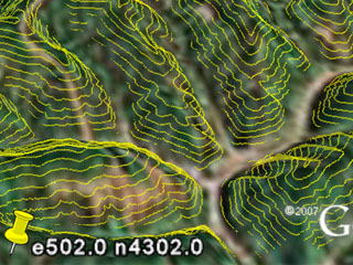
abstract:
We provide streaming tools that allow quick visualization of LIDAR data in
Google Earth. This is useful to quickly generate previews for large amount
of LIDAR data, to rapidly understand and verify their coverage, and to easily
present them within a popular geospatial context to a wide audience. An example:
we create the 10 by 8 tiling of 10 feet contours gilmer.kmz
(c,d) in only
20 minutes using less than 100 MB of main memory and no temporary disk space from
357 LAS files
(provided by West Virginia View)
that contain a total 156 million LIDAR points. Another, more interesting, example is
Mount Saint Helens
(c,d).
You can see that inside the vulcano the elevation of the Google Earth terrain is not correct. A reader of
gearthblog pointed out that the lava dome inside Mount St. Helens'
crater has grown recently
(apparently nearly 330 feet)
and that google earth may still be using older elevation data from the
Shuttle Radar Topography Mission
of 2000. Also check Toronto downtown
(c,d).
update:
We now also provide tools that generate raster DEM tilings
from LIDAR points for low turn-around time pre-viewing of large amounts of
LIDAR point data. An interesting example is the DSM with hillside-shading
based on the first returns from LIDAR points of Toronto downtown
(c,d).
The first thing you notice is how the perspective distortion in the satellite
images tricks you into missjudging the actual position of buildings. That this
also happened to the creators of the 3D buildings is quite evident. If you turn
on the 3D building layer you will notice that they do not always line up with
the footprints that are clear in our imagery. You can also see parking lots
and parks that have since turned into building or building sites. It's also fun to try and find details
that are hidden in the satellite images ... such as the other covered walkway in
the city hall building.
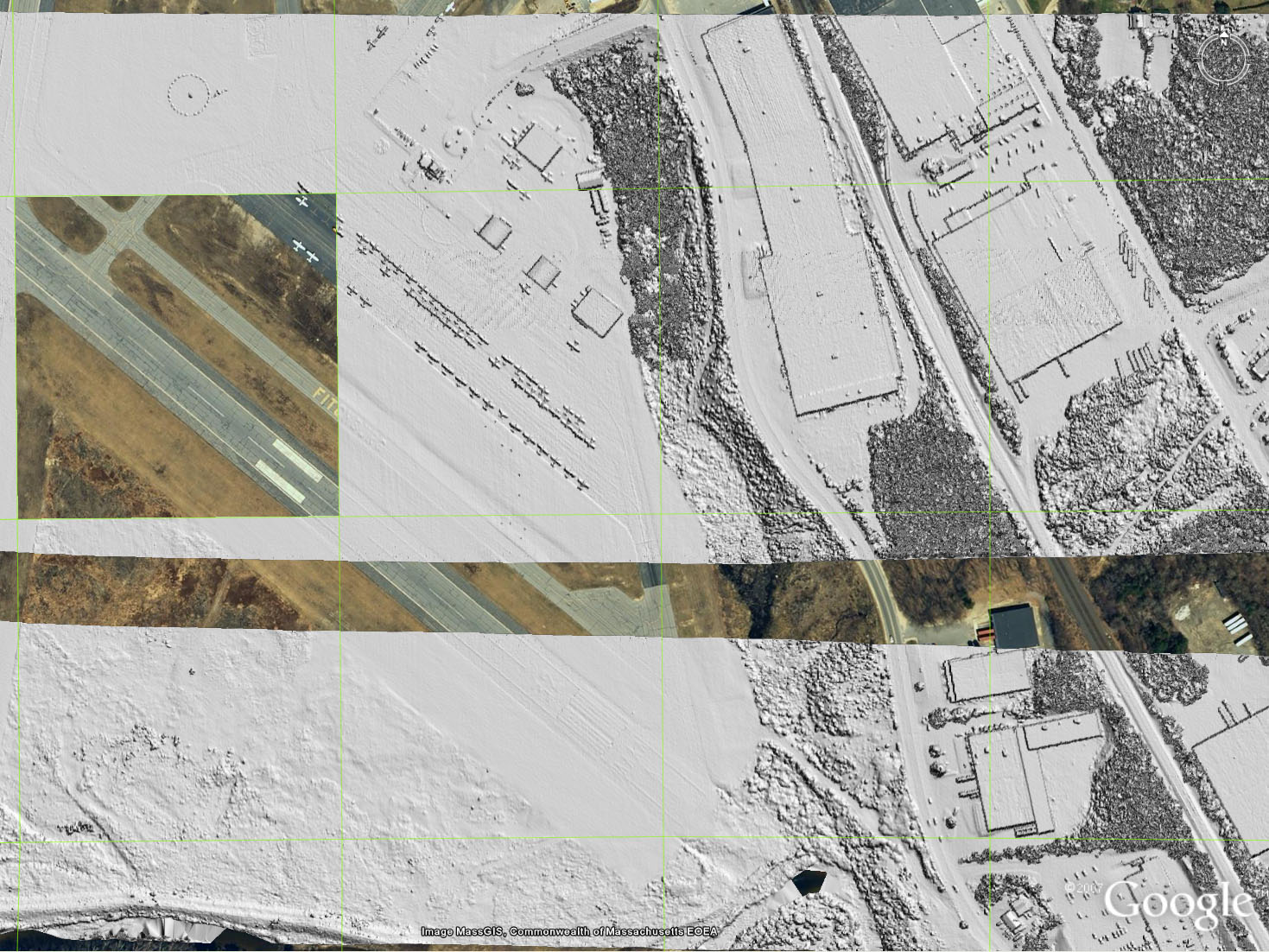
Other examples are New Orleans downtown (c,d) (bare earth, see for yourself where those leeves are), Fitchburg airport (c,d) (first returns, check out how the planes have moved), Mount Saint Helens (c,d) (bare earth), Baisman Run (c,d) (bare-earth, amazing how you can suddenly "see" through the canopy), Gilmer county (c,d) (bare-earth, go find something interesting), UC Santa Barbara (c,d), and Sydney (d). These DEMs are derived from a seamlessly generated streaming TIN of the LIDAR points as described here.
details:
Here is the command line that creates gilmer.kmz
(c,d) from 156
million LIDAR points stored in 357 files:
spfinalize -i gilmer.files -lof -ilas -level 8 -ospb | spdelaunay2d -ispb -osmb | tin2iso -ismb -range 200 450 10 -oslb | slclean -islb -oslb -length 5 | slsimp -islb -oslb -area 0.7 | sl2sl -islb -okml -tiling_nllsxy gilmer 500000 4302000 2000 10 8 -utm 17S -ellipsoid 23
The first module spfinalize.exe (README) reads the points from a list of files (-lof) in gilmer.files that can be found here and that are in LAS 1.x format (-ilas), finalizes them on a 256x256 grid (-level 8), and outputs them in a streaming binary point format (-ospb) to the second module.
The second module spdelaunay2d.exe (README) reads the points in streaming binary format (-ispb) as they are produced by the finalizer and Delaunay triangulates them with the Streaming Delaunay algorithm described in SIGGAPH 2006. It immediately starts to output the triangulation in a binary Streaming Mesh format (-osmb) and pipes it to the third module.
The third module tin2iso.exe (README) reads the triangulation from the binary streaming mesh format (-ismb) as it is produced by the streaming triangulator, extracts elevation contours every 10 units (here: meter) between 200 and 450 (-range 200 450 10) and outputs the resulting lines in a binary streaming line format (-oslb) to the fourth module.
The fourth module slclean.exe (README) reads the contours in binary streaming line format (-islb) as they are produced by the extractor, discards all contours that are shorter than 5 units (here: meter) (-length 5), and outputs others as soon as their length is determined as being above the cutoff in a binary streaming line format (-oslb) to the fifth module.
The fifth module slsimp.exe (README) reads the contours in binary streaming line format (-islb) as they are output by the cleaner, removes all 'bumps' (i.e. pairs of two subsequent line segments) that have less than 0.7 square units (here: square meter) in area (-area 0.7), and outputs the simplified contours in a binary streaming line format (-oslb) to the sixth module.
The sixth module sl2sl.exe (README) reads the contours in binary streaming line format (-islb) as output by the simplifier and tiles them into x=0..9 by y=0..7 separate files called gilmer_00x_00y.kml with (500000,4302000) being the lower left corner of the tiling and with each tile being 2000 units (here: meters) long and wide (-tiling_nllsxy gilmer 500000 4302000 2000 10 8); each tile is stored in Google's KML format (-okml). KML uses a longitude [degree], latitude [degree], elevation [meter] representation we need meta data to convert the LIDAR data to a correctly georeferenced representation. The LIDAR data was in UTM format and we specify 17S as the zone (-utm 17S) and WGS-84 as the ellipsoid (-ellipsoid 23).
Because our elevation data is much more precise than the terrain data used by Google Earth the isolines don't align perfectly with the terrain. Because of the lower resolution ravines in GE are less deep, so our isolines run below the GE terrain, and ridges in GE are less tall, so our isolines float above the GE terrain.
If you work with LAS or LIDAR you may also be interested in our LAStools.
tools: (updated on October 17th, 2007)
spfinalize.exe reads the points from a list of files (-lof) saint_helens.files in LAS 1.x format (-ilas). Because the LIDAR points are originally provided in a less efficient ASCII format we first convert them with txt2las.exe of our LAStools package.
example LIDAR data in LAS format:
related publications:
related downloads:
You may use the binaries and source code for non-commerical purposes only.