


Line fitting. (assignment)
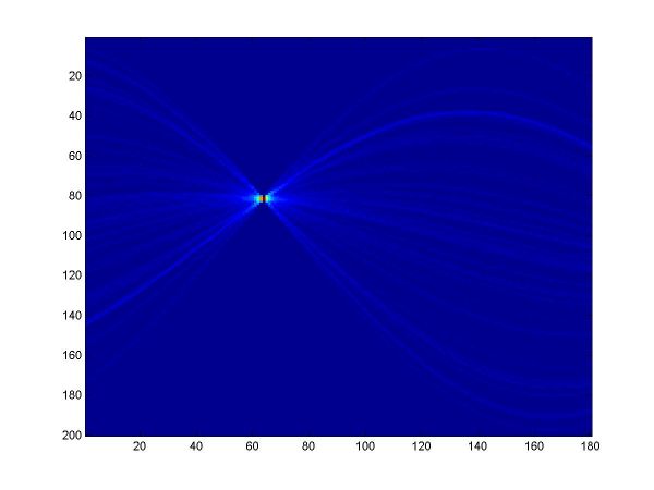
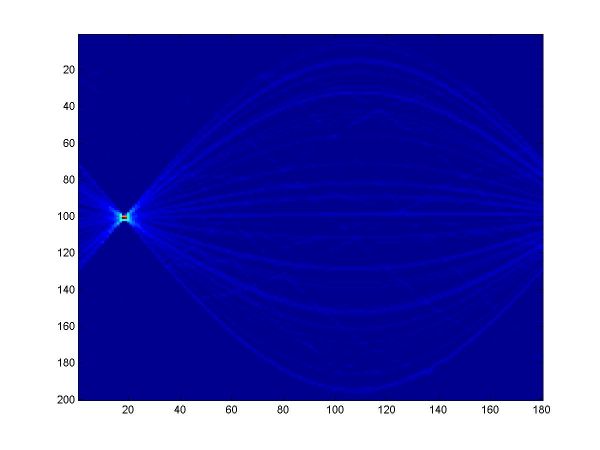
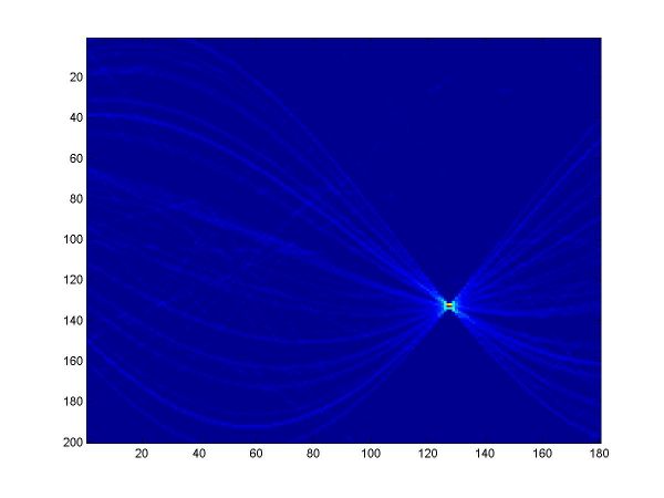
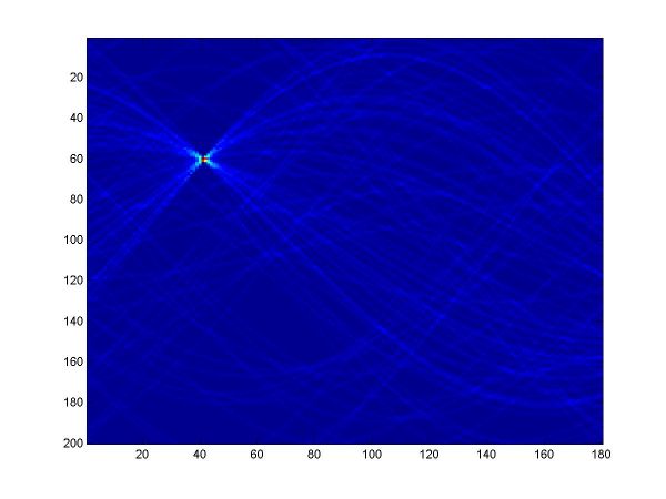
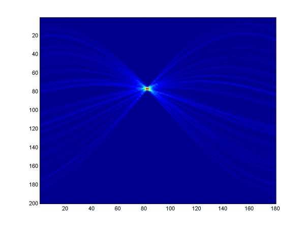
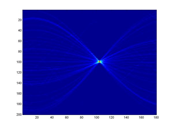
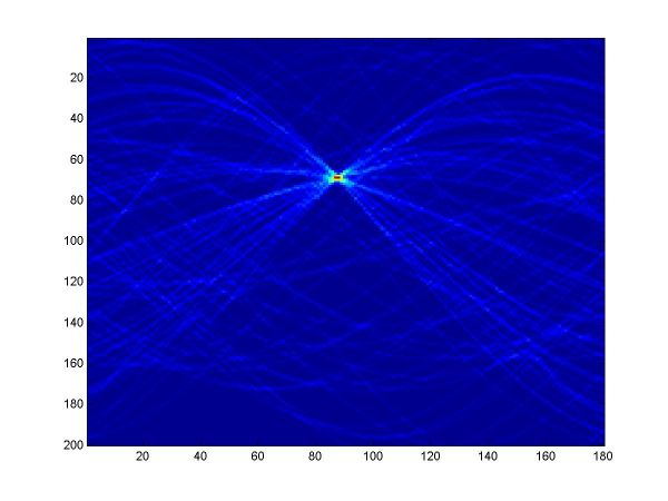
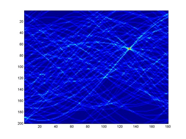
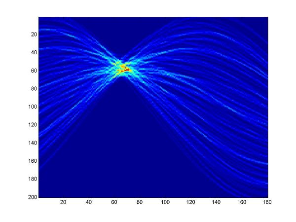
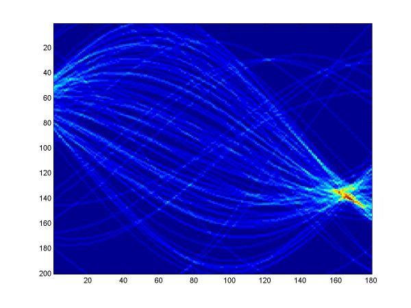
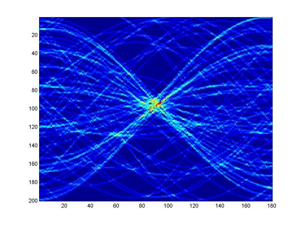
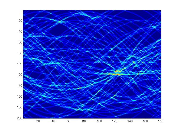
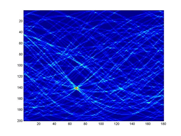
For the first part, I implemented a classic Hough transform algorithm in MatLab (Hough.m). It takes as parameters a set of points generated by the provided datagen.m, a distance threshold, and the discretizing parameters for the angle and distance domains. I chose the distance threshold empirically, setting it to 0.01. Larger values produce thicker curves in the Hough transform image. I discretized the angle domain to 180 intervals, and the distance domain to 200 intervals.
For the second part, I implemented a variation of the RANSAC algorithm (ransac.m) as described in the class slides. The pseudocode of my implementation is as follows:
For the distance threshold used to decide if a point is an inlier, I used the value suggested in class, sqrt(3.8)*sigma. For the threshold used to decide if the model is good enough to refit the data, I tried several alternatives. I ended up using inliers*(10*(sigma*100+3))/100, knowing that sigma=0, 0.01 or 0.05, and the total number of points is 100. This formula requires that more inliers fit the model if sigma is larger.
For the third part, I implemented a variation of the E-M algorithm (em.m) as described in the class slides. For the E phase I simply computed the probabilities using the provided formula (valid only for sigma~=0). For the M phase, I modified the provided routine linefit.m into linefit2.m to take into account the probabilities.
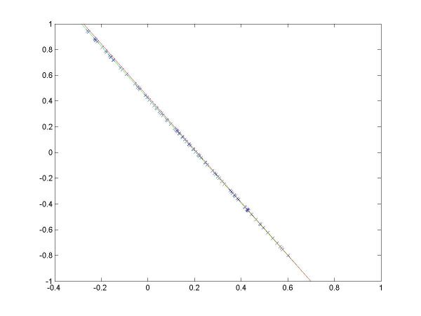
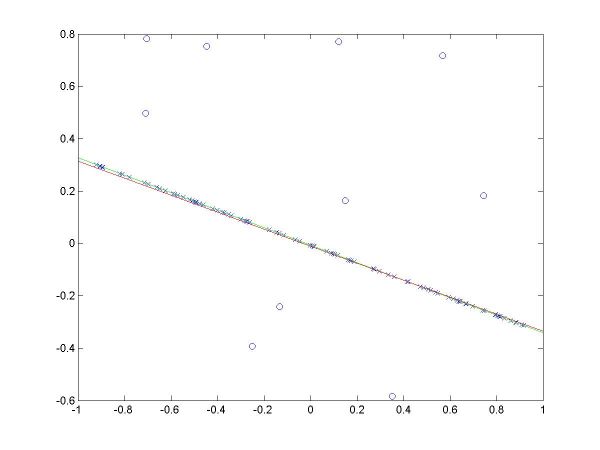
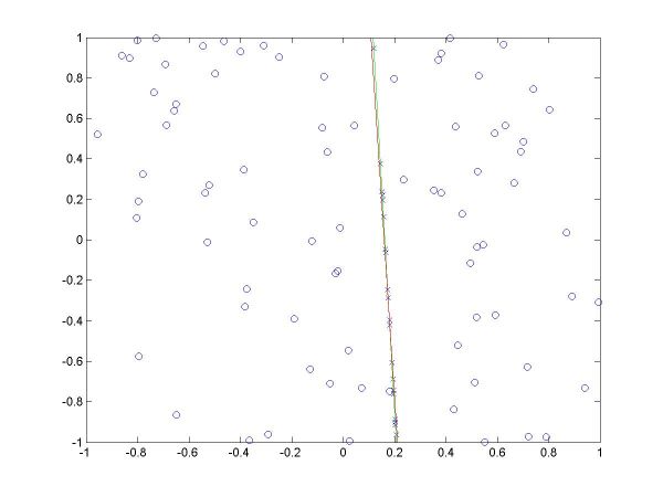
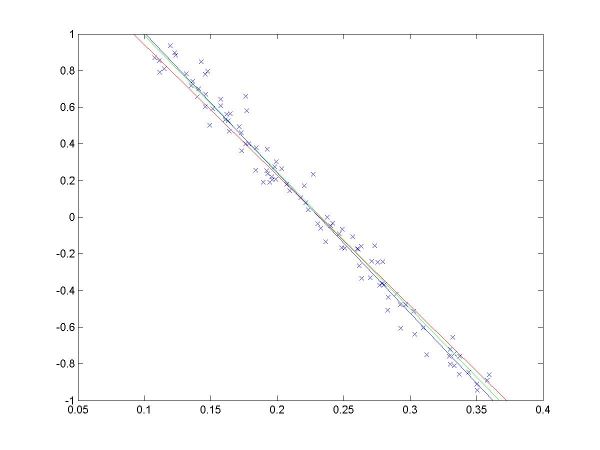
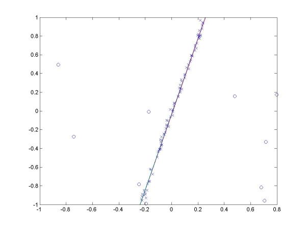
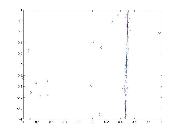
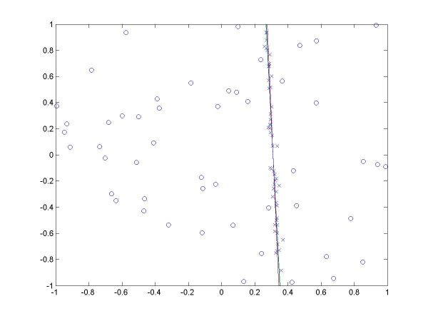
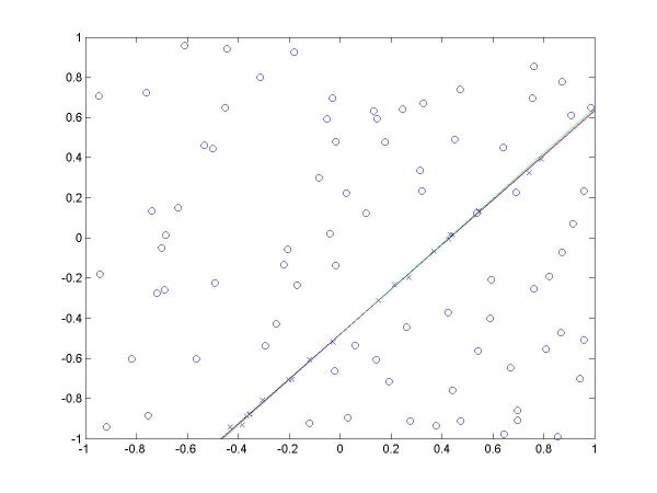
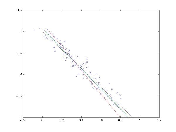
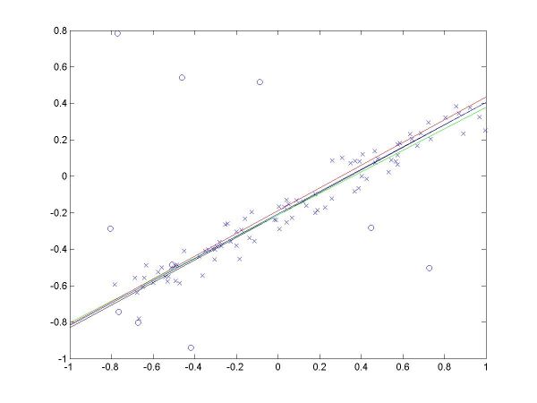
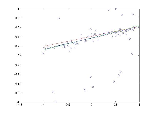
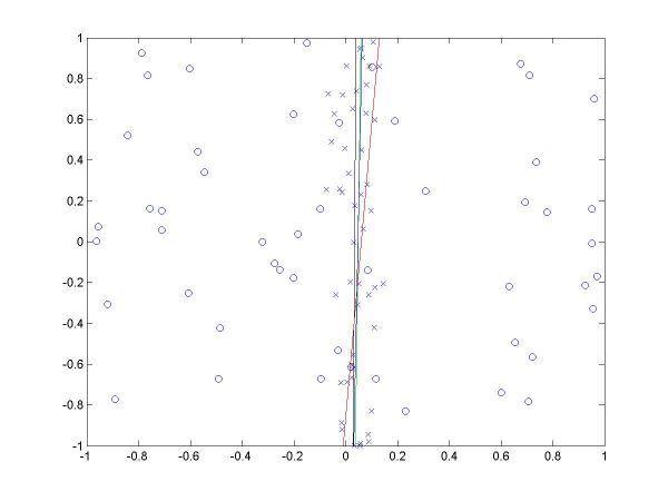
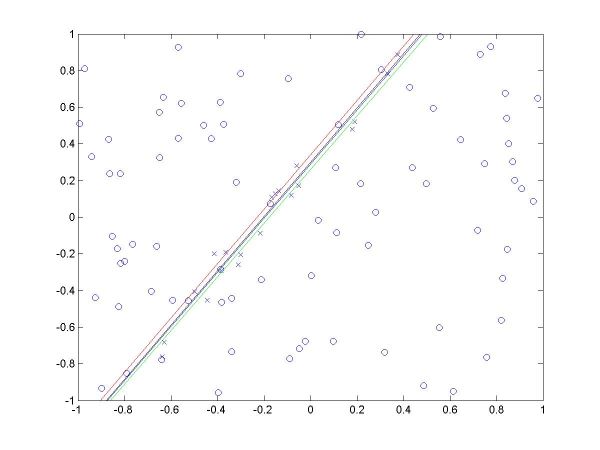
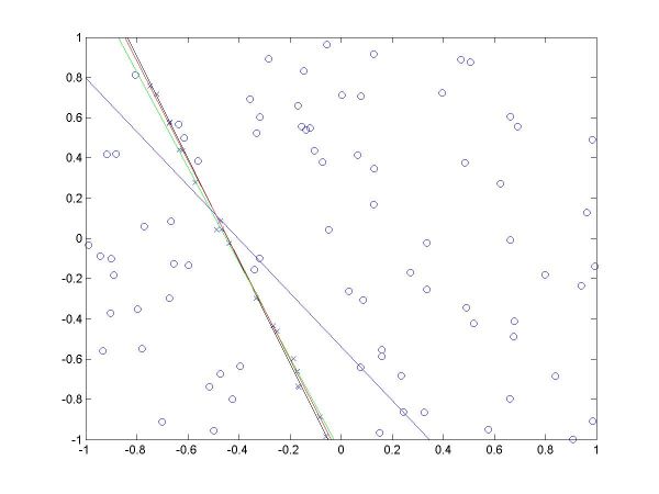
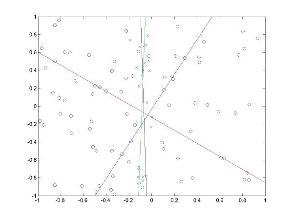
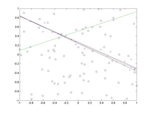
I have plotted all the algorithms in the same coordinates (using em.m, and two line drawing routines, drawline.m and drawline2.m), to be able to compare their performances. The Hough lines are red, the RANSAC lines are green, the E-M lies are blue, and the true lines (as generated) are black. As the formula for the probabilities is invalid for sigma=0 (1/2*sigma=infinity), the E-M plot is missing from the corresponding data. The table below shows the results for the required values of sigma and the number of inliers (click on each image for a larger version).
| inliers | 100 | 90 | 80 | 50 | 20 | |
|---|---|---|---|---|---|---|
| sigma |
|
|||||
| 0 | plots | |
|
|
|
|
| Hough | |
|
|
|
|
|
| 0.01 | plots | |
|
|
|
|
| Hough | |
|
|
|
|
|
| 0.05 | plots | |
|
|
|
|
| Hough | |
|
|
|
|
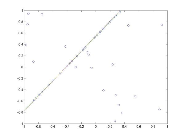
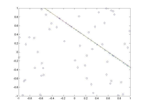
For more than 50 inliers, all three methods behaved well, and their results were not much different than the true line. However, for only 20 inliers, good results like the ones shown in the last column above were random, their frequency being inverse proportional to sigma (the larger sigma, the less likely to obtain a good result). The table below shows a few such cases.
| sigma | 0.01 | 0.01 | 0.05 | 0.05 | 0.05 | |
|---|---|---|---|---|---|---|
| inliers |
|
|||||
| 20 | plots | |
 |
|
 |
 |
| Hough | |
 |
|
 |
 |
The second column shows a case where E-M has drifted from both Hough and RANSAC, into a local minima, for sigma=0.01. The fourth column shows a case where Hough misses, RANSAC behaves well, and E-M worsens the RANSAC solution (for sigma=0.05). The fifth column shows a case where Hough and E-M give good results, but RANSAC misses (for sigma=0.05).