
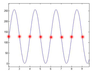
What is happening here is very simple. Basically it is a matter of sampling a signal that is close in frequency to the rate at which we are sampling the signal. Specifically, when f=0.5 the signal has half the frequency of our sampling rate. When the signal's frequency is half the frequency we are sampling at, each sample hits the sine wave at the spot where it crosses zero. Therefore the sampled signal looks like a flat line, or in image form, a constant gray across the entire image. This can be seen in Figure 1. Figure 2 depicts how the samples hit the signal to create the flat image. The blue sine wave is our theoretical analog signal before it is sampled and the red dots indicate where the samples are taken.
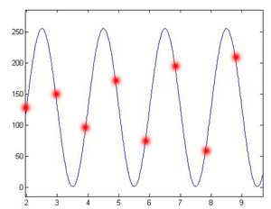
When we sample at a slightly lower frequency (0.495) we see that our samples hit successively different spots on the signal giving the appearance of sampling a much lower frequency signal (Figure 3). Figure 4 depicts how the samples hit the signal in this case.
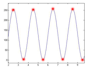
If we shift the phase of the signal by pi/2 when the frequency is 0.5, we might expect to see something very similar to the first image, however, we get something very different. This occurs because the samples are now hitting the alternating peaks of the signal instead of all the spots where it hits zero. Figure 5 is what is produced when this occurs and Figure 6 depicts what is happening with the samples.
|
|
| Figure 1. Sine f=0.5 | Figure 2. Samples f=0.5 |
 |
 |
| Figure 3. Sine f=0.495 | Figure 4. Samples f=0.495 |
 |
 |
| Figure 5. Sine f=0.5 with pi/2 phase shift | Figure 6. Samples f=0.5 with pi/2 phase shift |
My implementation of the function that creates an NxN matrix that represents the DFT can be found here - fftm.m. This matrix is not normalized and so here is a second function that creates an orthonormal DFT matrix - fftm_norm.m I can demonstrate that the matrix created by fftm_norm is orthonormal by showing that all its rows are normalized and that each row is perpendicular to all the other rows. Orthogonality is shown with a series of dot products, which should all equal zero. Due to rounding error with floating points, the answers show up as very very small numbers and not exactly zero. A diary of a demonstration that the matrix is orthonormal can be found here - orthonormal.txt
I compared the answer I get from doing M*X and the answer I get from using MATLAB's fft(X). For my unnormalized matrix the answer agrees everywhere. They have the same frequency responses and even the same magnitude peaks. When I normalize my matrix, I get the same frequency response but the peaks have less magnitude. But it is still essentially identical as fft(X) only scaled by some normalization factor.
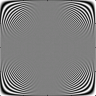
Figures 7 and 8 respectively represent the real and imaginary parts of the DFT matrix. We can learn quite a lot from examining these images. First, they appear very similar. This is because the real part represents cosine whereas the imaginary part represents sine. Therefore the only difference between the two images is the phase. The phase difference is best viewed at the corners where the starting and ending points of the waves differ, and at the center where the phase difference causes the centers of each image to have opposite colors. Another interesting thing we notice when examining the image is that it is very symmetric. The real image is symmetric across its central axes, whereas the imaginary image is more of a mirror effect. It is the inverse of itself on either side of the central axes. This is explained again by phase, because cosine is symmetric about its half period, where sine is mirror of itself about its half period. The symmetry itself is actually quite interesting too. Even though the frequency of the waves increase as we go down the vertical axis, once we reach the midpoint, the frequency actually appears to decrease. This is caused by the same effect as seen in Part 1. The wave's frequency is exactly half of the sampling frequency at the midpoint. Due to the Nyquist limit, this is the highest frequency we are able to sample. As the frequency goes past this limit, it begins to alias and appear to be a different lower frequency, until it again reaches what appears to be a zero frequency at the bottom. Infact this is a frequency equal to the sampling frequency, so the samples hit the wave at the same point every time making it appear as though it was a frequency of zero. This symmetry also explains why frequencies show up twice (once on each side) when you do the Fourier Transform.
 |
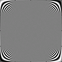 |
| Figure 7. Real part of FFT matrix | Figure 8. Imaginary part of FFT matrix |
The Fast Fourier Transform is based mostly in magic, which makes it difficult to explain its speed using mathematics and scientific reasoning. Despite this fact, I will try anyways. In reality, FFT uses nothing more than a mathematical trick to obtain its efficiency. First, it does not compute out a matrix like we did, as this requires a large amount of memory and ensures a computational time on the order of N^2. Instead, it relies on a divide and conquer approach to reduce the computation time down to an order of N log2 N. In 1942, Danielson and Lanczos found that the discrete Fourier transform of length N can be broken down into the sum of two DFTs of length N/2. These two sub sets are actually the even numbered and odd numbered components of the original series of data. This process of subdividing can be repeated over and over until we are doing transforms on data of length one. The transform of length one is a simple matter of putting the input data into the appropriate output slot.
Furthermore, there is a trick that can be applied to increase the efficiency of book-keeping for this recursive algorithm. If we label each subdivision with an 'e' if it is the even subdivision, and an 'o' if it is an odd subdivision, we can begin to expand the recursion out completely. This will give us a series of single transformations, each with some label denoting the series of even or odd subdivisions used to get to that element. For example, the first element in the data should end up with a label that is a bunch of e's log2 N in length. It turns out that if we take these labels, reverse the order of the pattern and convert e's to 0's and o's to 1's, we will have a binary value to tell us where that element belongs. The trick therefore is to take our input data, and rearrange it based on the bit-reversed order of its position in the series. Figure 9 demonstrates how the bit-reversal process works. As can be seen it is very simple and can be implemented very efficiently. Clearly one could imagine implementing this in N time or less, meaning it does not hurt the overall time of the algorithm. Now, all the points represent the single-point transformations. All that needs to be done is combine everything together by combining adjacent pairs recursively (so that we get two-point transformations, then four-point transformations, etc.) Each combination can be done on the order N time, and there are log2 N combinations, giving a total time on the order of N log2 N.
Therefore, the entire FFT algorithm has two parts. The first part involves sorting the data into the bit-reversed order. This part is efficient because it does not require extra memory. All that needs to happen is the swapping of pairs of data. You always swap pairs because the bit-reversal of one location is the bit-reversal of that location, so those two points just swap places. The second part of the algorithm involves a loop and two nested loops. The outermost loop performs the combinations to create transforms of length two, four, etc. This loop takes log2 N time. The first inner loop covers the sub-transformations that have already been calculated, while the second inner loop covers each element of the sub-transformation and implements the Danielson-Lanczos Lemma. As a side note, the efficiency of this algorithm can be further increased by only calculating sines and cosines at the outer loop, and using a recurrence relation to get sines and cosines of multiple angles in the inner loops.
Page I used as a reference to learn about FFT can be found here. It does a much better job of explaining the FFT than I do. It also gives some pseudo-code one could use to implement the FFT on their own.
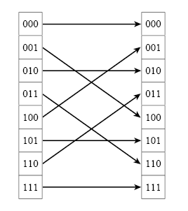 |
| Figure 9. Bit-reversal reordering |
Grading information and comments can be sent to  .
.