to COMP 205 Homework 2 Jan 21, 1998, Due: Jan. 28, 1998

Problems

1. (15 points) We are given a order polynomial :

   

   where is a root and is the coefficient of the high-order term. Consider the following procedure for evaluating the polynomial:

   

   Show that the relative error in evaluating a value is: where .

   Solution:

   We make the assumption that

   

   where , and where is our machine epsilon. Then our computed value is

   

   where the is the relative error on the product with , and the are the errors for each of the d - 1 products in the product term. Further, for each difference, we have , so our computed value is

   

   and if we don't differentiate between the different s, this gives

   

   and by our linear approximation,

   

   which gives the relative error bound we sought.

2. ( 15 points) Consider the following procedure to solve a linear system of equations:

   

   

   

   

   Show by means of a numerical example that Cramer's rule is not backward stable. Hint: choose the matrix nearly singular and . Your numerical example can be done by hand on paper (for example with 4 decimal digit floating point), on a computer, or a hand calculator. You should clearly explain why Cramer's rule is not backward stable. Is Cramer's rule forward stable?

   Solution:

   The key here is to see that it is the determinant computation and its possibility for catastrophic cancellation and loss of significant digits that renders Cramer's rule a bad method for linear system solving. We will chose a matrix which is nearly singular, but still well enough conditioned that Gaussian elimination with pivoting can find a good approximate answer, and see how poorly Cramer's rule can perform. Consider the linear system

   

   This has the exact solution and using Gaussian elimination with pivoting, with 4-decimal floating point, we can compute this answer accurately. Using Cramer's rule, however, we compute

   

   

   

   From these, we compute and . We can see right away that the forward error is rather awful. To compute the backward error, we consider this new to be the correct solution, and seek the perturbed problem that it solves exactly. We can keep fixed and simply compute a new by

   

   This gives a relative backward error (using the vector norm) of

   

3. 1. How do you account for the asymmetry between Algorithm I and Algorithm II? Using a different positive value of would not solve the asymmetry problem. Try to explain your answer geometrically. (10 points)

      Solution:

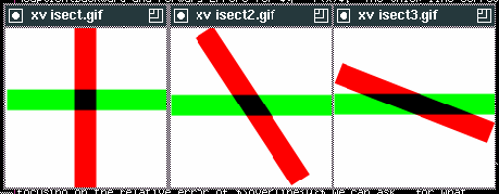
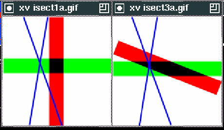
      The key to understanding the asymmetry lies in visualizing the test that's taking place. A point of intersection between two of the lines is computed, and then this is tested against each of the other two lines in turn, to see if it lies within of that line. This gives us an accept-region of width about each of the two lines, and the intersection of the accept-regions is the area within which our test will return INTERSECT. Since the shape/area of this INTERSECT region will depend on the angle between the lines and on their orientation, use of such a test clearly leads to an algorithm which depends on which pair of lines is chosen. (See diagrams on next page)

   2. Your goal is to modify the algorithm to account for the asymmetry for all pairs of four lines. Given four lines, for all input permutations (24 permutations in this case), the algorithm should give a consistent answer using floating point arithmetic. You can assume that no two lines are parallel to each other. Furthermore, we would like to use a positive (non-zero) value of . (10 points)

      Solution:

      There are a number of correct ways to eliminate asymmetric dependence of test results on the order of the input.

      1. Simplest---and requiring the least modification to the present algorithm---would be to enforce a ordering on the inputs, based on any unique sort criterion, so that any permutation of the input would be consistently put in a single input order. This eliminates the asymmetry, but does nothing to deal with the inconsistencies between trials caused by test regions that change shape.

      2. A brute force solution would be to compute all six points of intersection, and see if the maximum distance between any two pairs is less than . This eliminates both input asymmetries and test inconsistences, at the cost of six intersection computations rather than one.

      3. An intermediate solution might be to sort the inputs (eliminating asymmetries), then check the point of intersection between the first line and the three others, and if the three intersection points are all within , return an INTERSECTION. This requires only 3 intersection computations rather than six. One might chose the line most orthogonal to the other 3 for the test line, to achieve the most stable result.

  
Figure 1: Accept-region intersections of width between two lines.

  
Figure 2: Ambiguous test results of lines with unaltered intersection points.

• About this document ...