Testing least squares fitting of a matrix subdivision surface
This matlab document shows the results of running my new code for the subdivision surfaces -- specifically, to do least squares fit for the hidden p values at each triangulation vertex so they best fit sample data.
I'm using the data from Wenjie's GUI, although there is a little bit of work required to get these routines to mesh with the GUI itself.
I run on the same samples with two slightly different triangulations and plot graphs and histograms comparing the equations, solutions, and residuals, then close with some comparison with the older code.
I'm not testing other, less regular triangulations; there remain some questions about the matrices used, which I close with.
Contents
- DATA: Using the original mesh and data from Wenjie's GUI
- Making equations
- Exploring the coefficients in A: pattern of non-zeros
- Exploring the coefficients in A: histogram of -log of nonzero coefficients
- Exploring the coefficients in A: Number of equations per variable
- Number of equations per variable,
- DATA: Adjusted mesh
- Exploring right hand side b for both data sets
- Exploring right hand side b, by triangle.
- SOLUTION: P values calculated from least squares fit
- Trimesh with Ps
- Trimesh with sign(P)*log (1+|P|)s
- RESIDUALS: Residuals by triangle
- Residuals plotted at sample points
- log(1+ residuals) at sample points
- COMPARING to evalBasisAll
- Display differences between bases
- Look for coefficients that were not used in the PLeastq basis.
- MATRICES & QUESTIONS
- Matrices for refinement
- Question: Matrices for adjusting ordinary points
- Questions: matrices for extraordinary points
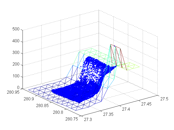
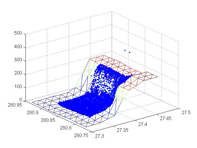
DATA: Using the original mesh and data from Wenjie's GUI
Our first look at the data. In the right corner, we just happened to hit a 200 meter outlier (perhaps a fish in the bathymetry data) which is going to hurt the quality of approximation for the triangles in that area.
load tempP
trimesh(TRI,x,y,z, 'FaceColor','none');
hold on
plot3(sx,sy,sz,'.')
hold off
X=x; Y=y; Z=z;
SX=sx; SY=sy; SZ=sz;
Making equations
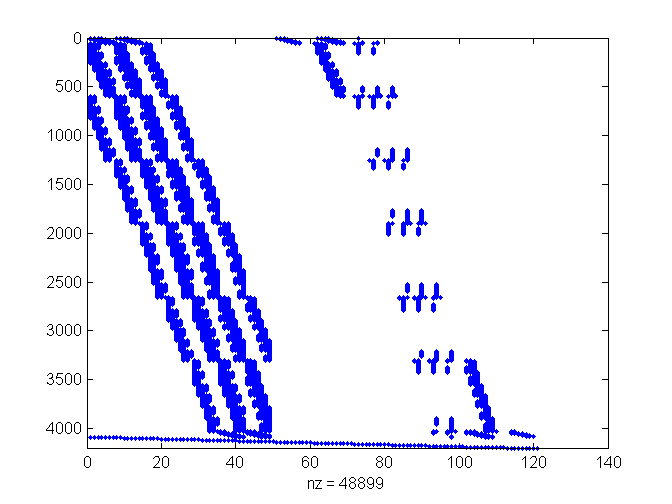
My function makes the linear system Ap=b directly to determine the p value for each triangulation vertex in the order given. A is a sparse matrix with column for each vertex and a row for each sample. I add the equations pi=0 so there is at least one equation for each variable, and to encourage the pis to be small.
Plot shows non-zero coefficients; rows are samples by triangle to give more structure.
tic;
[A,b,utri]=makeEquations(TRI,[x' y' z'],[sx' sy' sz']);
toc
tic;
P=A\b;
toc
[junk ix] = sort(utri); % for sorting samples by triangle
ix = [ix; ((length(ix)+1):length(b))']; % Don't forget added equations for p_i=0.
resid = A*P-b;
Elapsed time is 13.297149 seconds.
Elapsed time is 0.427774 seconds.
Exploring the coefficients in A: pattern of non-zeros
(rows grouped by triangle)
spy(A(ix,:))
axis fill;
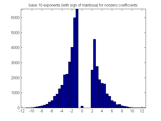
Exploring the coefficients in A: histogram of -log of nonzero coefficients
hist(-sign(nonzeros(A)).*log10(abs(nonzeros(A))),-12:.5:12)
title('base 10 exponents (with sign of mantissa) for nonzero coefficients')
set(gca,'XTick', -12:2:12)
axis tight
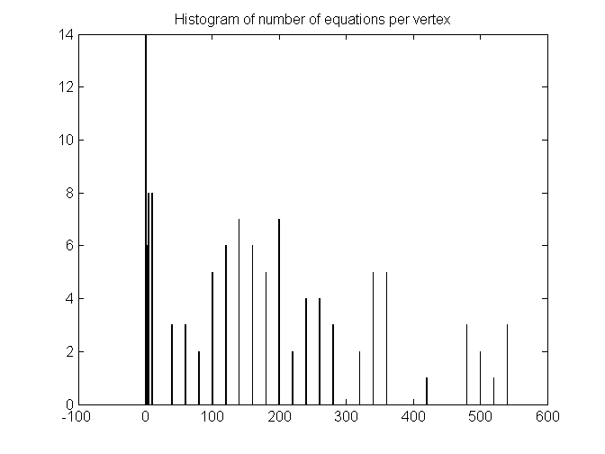
Exploring the coefficients in A: Number of equations per variable
Histogram of number of equations for each vertex's p value.
s = full(sum(A>0));
mxs = max(s);
[n0,xout] = hist(s, [0 1 2 3 4 5 10 20:20:mxs+20]);
bar(xout,n0);
title('Histogram of number of equations per vertex');
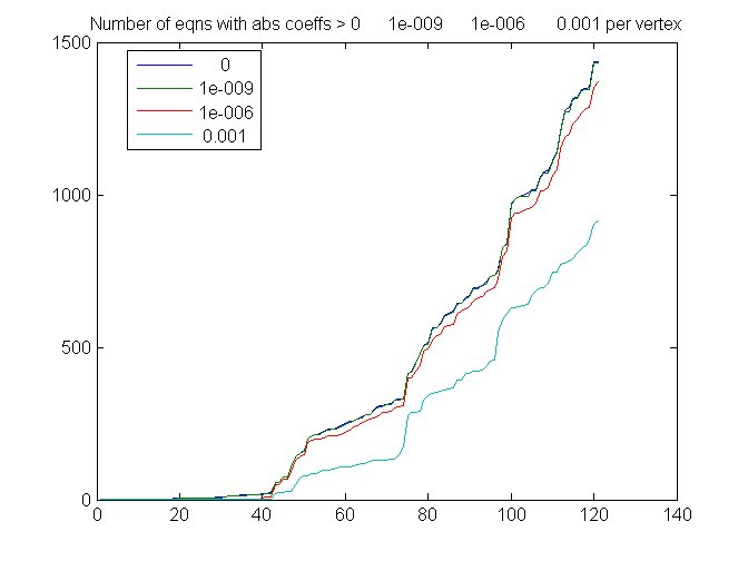
Number of equations per variable,
Counting only abs coefficients > various thresholds
thresh = [0 1e-9 1e-6 1e-3]'; % 0 already done
s = zeros(size(A,2), length(thresh));
for i = 1:length(thresh);
    s(:,i) = sort(full(sum(abs(A)>thresh(i))))';
end
plot(s)
legend(num2str(thresh),'Location', 'best');
title(['Number of eqns with abs coeffs > ' num2str(thresh') ' per vertex']);
DATA: Adjusted mesh
Minor adjustments avoid that outlier sample point.
load tempPadj
trimesh(TRI,x,y,z, 'FaceColor','none');
hold on
plot3(sx,sy,sz,'.')
hold off

tic;
[Aadj,badj,utriadj]=makeEquations(TRI,[x' y' z'],[sx' sy' sz']);
toc
tic;
Padj=Aadj\badj;
toc
[junk ixa] = sort(utri); % for sorting samples by triangle
ixa = [ixa; ((length(ixa)+1):length(b))']; % Don't forget added equations for p_i=0.
resadj = full(Aadj*Padj)-badj;
Elapsed time is 11.126211 seconds.
Elapsed time is 1.011667 seconds.
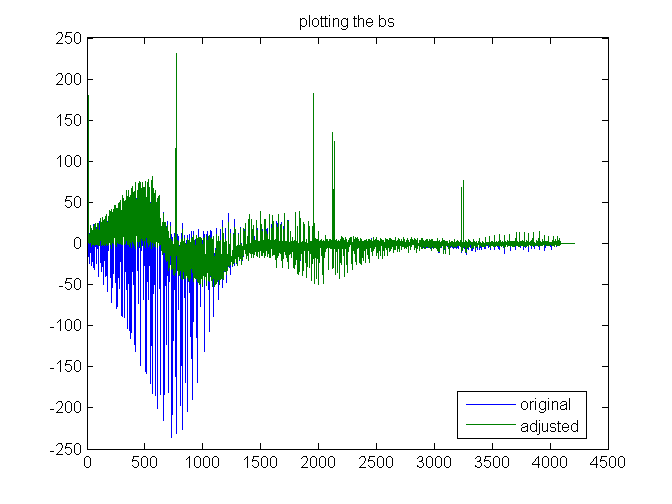
Exploring right hand side b for both data sets
The right hand side shows that in a few places the z value is not well predicted from the neighbors. original is blue, adjusted green.
plot([b badj])
title('plotting the bs')
legend('original','adjusted','Location','best')
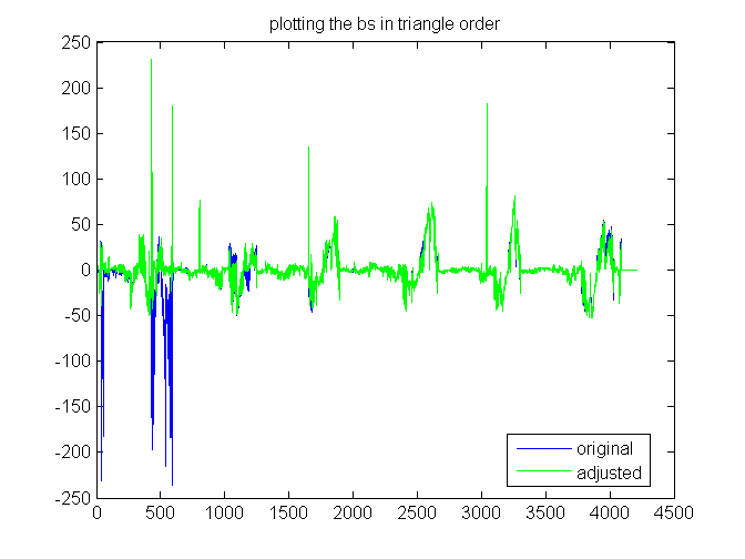
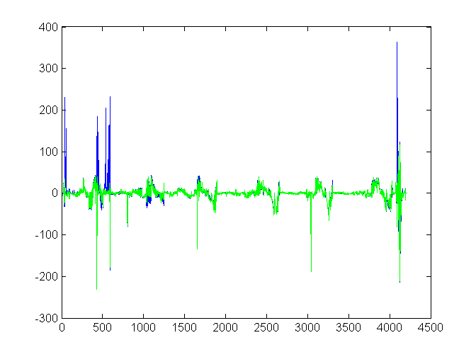
Exploring right hand side b, by triangle.
Same as the previous plot, but sorted by triangle. The right hand side shows that in a few places the z value is not well predicted from the neighbors. original is blue, adjusted green,
plot(b(ix))
hold on
plot(badj(ixa),'g-')
hold off
title('plotting the bs in triangle order')
legend('original','adjusted','Location','best')
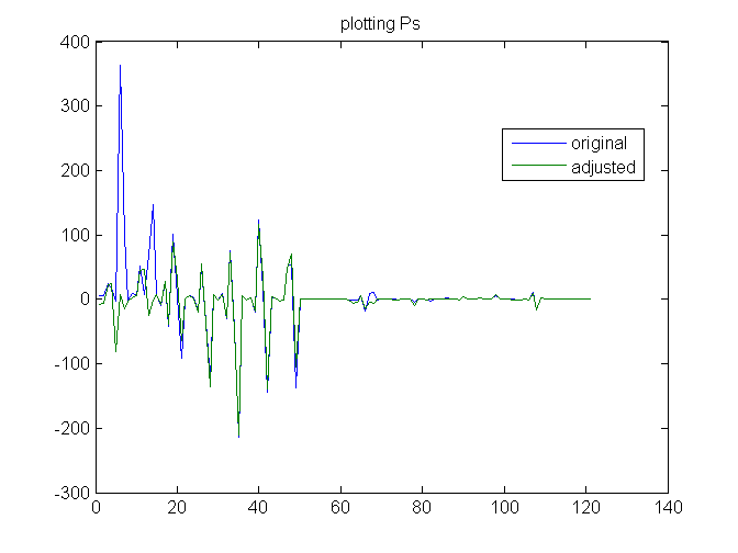
SOLUTION: P values calculated from least squares fit
plot([P Padj])
title ('plotting Ps')
legend('original','adjusted','Location','best')
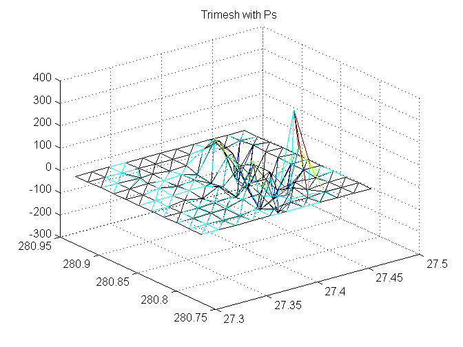
Trimesh with Ps
adjusted is black
trimesh(TRI,X,Y,P, 'FaceColor','none');
hold on
trimesh(TRI,x,y,Padj,'EdgeColor','k', 'FaceColor','none');
hold off
title('Trimesh with Ps');
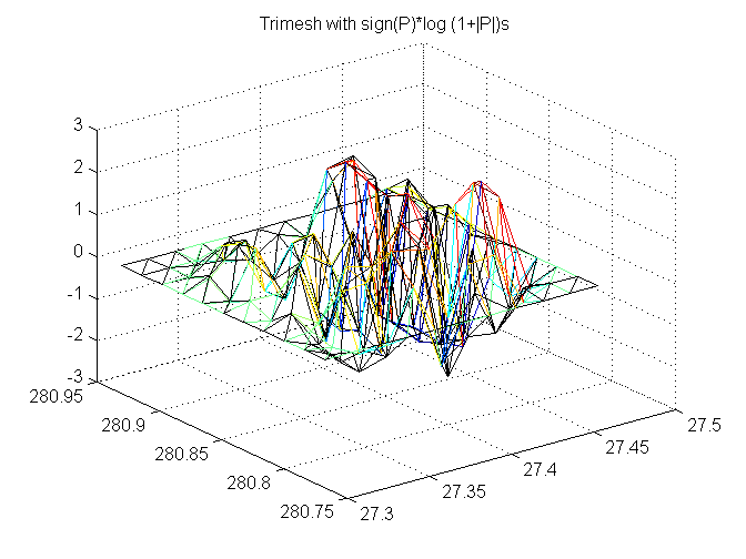
Trimesh with sign(P)*log (1+|P|)s
adjusted is black
trimesh(TRI,X,Y,sign(P).*log10(1+abs(P)), 'FaceColor','none');
hold on
trimesh(TRI,x,y,sign(Padj).*log10(1+abs(Padj)),'EdgeColor','k', 'FaceColor','none');
hold off
title('Trimesh with sign(P)*log (1+|P|)s')
RESIDUALS: Residuals by triangle
Blue is original; green is adjusted.
plot(resid(ix))
hold on
plot(resadj(ixa),'g-')
hold off

sumAbsResid = [sum(abs(resid)) sum(abs(resadj))]
sumAbsResid =
        39080        30239
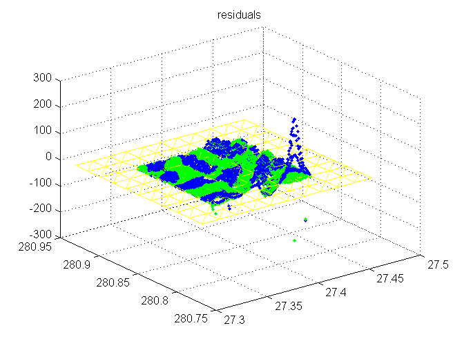
Residuals plotted at sample points
Blue is original; green is adjusted. Flattened trimesh (adjusted) for context.
trimesh(TRI,x,y,zeros(size(x)),'EdgeColor','y', 'FaceColor','none');
hold on
plot3(SX,SY,resid(1:length(SX)),'b.')
plot3(sx, sy, resadj(1:length(sx)), 'g.')
hold off
title('residuals')
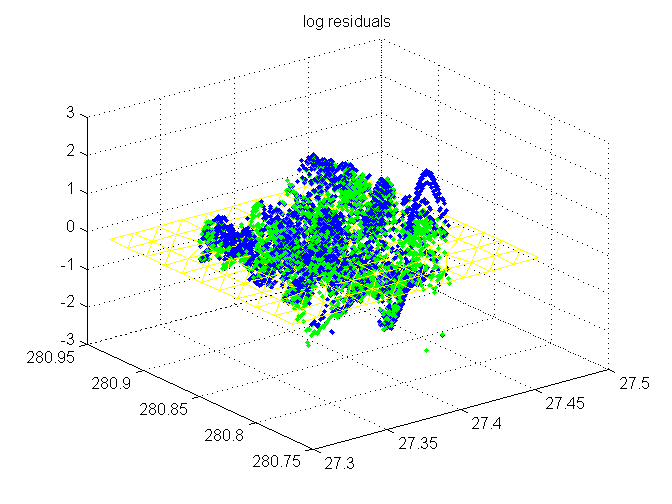
log(1+ residuals) at sample points
Blue is original; green is adjusted Flattened trimesh (adjusted) for context.
trimesh(TRI,x,y,zeros(size(x)),'EdgeColor','y', 'FaceColor','none');
hold on
r = sign(resid).*log10(1+abs(resid));
plot3(SX,SY,r(1:length(SX)),'b.')
r = sign(resadj).*log10(1+abs(resadj));
plot3(sx,sy,r(1:length(sx)),'g.')
hold off
title('log residuals')
COMPARING to evalBasisAll
The PLeastsq code used evalBasisAll to find the basis. It returns a data structure that we can try to compare to the p coeffients in the matrix A.
In order to compare bases, we use a modified version of our code to compute a matrix with only four levels of subdivision, no early exit, & snapping at lowest level (to triangle center instead of barycentric.)
The new code is faster, and has already built the matrix, which takes about 10% additional time after evalBasisAll.
trythese =  1:length(sx); %500;%:500:4000; % set to a sample for a quick check

disp('evalBasisAll time')
tic
val=evalBasisAll(TRI,x,y,[sx(trythese)' sy(trythese)']);
toc
% tic
% Pold=findP2(TRI,x,y,z,sx,sy,sz,meshSize);
% toc

disp('makeEquationsSnap time')
tic;
AA=makeEquationsSnap(TRI,[x' y' z'],[sx(trythese)' sy(trythese)' sz(trythese)']);
toc
evalBasisAll time
Elapsed time is 280.890742 seconds.
makeEquationsSnap time
Elapsed time is 7.625737 seconds.
Display differences between bases
val: the value matrix contains 3 columns per sample point. For sample i, we care about * col (3*i-2)= triangulation vertex index * col (3*i) = p coefficient for that index
If no problems are displayed after the heading, we're all good. Note: this clears matching coefficients, so to rerun, you also need to rerun the previous cell.
fprintf('\n differences to nonzero basis elements\nSmplPt vert row     basis        coeff        diff\n');
for r = 1:length(trythese)
    for i = 1:size(val,1)
        v = val(i,3*r-2);
        if v>0
          if abs(AA(r,v) - val(i,3*r))>1e-9
              fprintf('%5d %3d %3d %12f %12f %12f\n',...
                  r,v,i,val(i,3*r),AA(r,v),val(i,3*r)-AA(r,v));
          end
          AA(r,v) = 0;
        end
    end
end
 differences to nonzero basis elements
SmplPt vert row     basis        coeff        diff
Look for coefficients that were not used in the PLeastq basis.
Too many to display, but they all seem to be for vertices that don't have complete two-rings in the mesh, but do have complete one-rings, so can still be used.
[ia,ja,va] = find(AA(1:length(trythese),:));
disp('Vertices for which a basis coefficient was not used by PLeastsq')
unique(ja')
%fprintf('\n\nzero basis elements that are used by makeEquations\nSmplPt vert    coeff\n');
% clear res
% if ~isempty(ia)
%     res(1,:) = ia(:);
%     res(2,:) = ja(:);
%     res(3,:) = va(:);
%     fprintf('%5d %3d %12f\n', res)
% end
Vertices for which a basis coefficient was not used by PLeastsq
ans =
  Columns 1 through 8
    50    51    52    53    55    56    57    61
  Columns 9 through 16
    62    63    64    65    66    67    68    69
  Columns 17 through 24
    72    73    74    77    78    79    81    82
  Columns 25 through 32
    83    85    86    87    88    89    90    92
  Columns 33 through 40
    93    94    96    97    98    99   101   102
  Columns 41 through 48
   103   104   105   106   107   108   109   110
  Columns 49 through 54
   113   114   115   119   120   121
MATRICES & QUESTIONS
Below are the matrices I'm using, from the PLeastsq code, plus some questions about them.
Matrices for refinement
Given four points of a diamond, 1234, with edge joining 13, The z,p parameters of a new point is created on the edge by [z1 p1; z3 p3] * Bmx + [z2 p2; z4 p4]*Cmx. Thus, 2*Bmx + 2*Cmx should have a_11 = 1 so that the new z coordinate keeps is relative position if the points are translated in z.
Bmx = [3/8, 0; -47/512, 69/512]; % refine
Cmx = [1/8, 0; -17/512, -5/512];

2*Bmx + 2*Cmx
ans =
            1            0
        -0.25         0.25
Question: Matrices for adjusting ordinary points
These matrices adjust the center of a one-ring. I'm surprised that the contribution of p is entirely negative; also, I would expect that the contribution from refined vertices might match the contribution from adjusting (perhaps divided by 3, since there are 3 times more new vertices created by refinement.)
Pmx = [1, -435/256; 0, -91/256]; % avg
Dmx = [0, 145/512; 0, -45/512];

Pmx + 6* Dmx
ans =
            1            0
            0     -0.88281
Questions: matrices for extraordinary points
- I would have expected this to match the above in the degree n=6 case. Why doesn't it?
- Is there an easy explanation for the sign change in the second column as the degree increases?
- The total increase in number of vertices remains about 3 times, so there should be some relationship to that...?
for n = 3:10
    an = 5/8 - ( 3/8 + 1/4 * cos( 2*pi / n ) )^2;   % avg, deg~=6
    Qnmx = [1, an*(-145/31); 0, -an];               %<== P
    Anmx = (512/31) * an * Dmx;                     %<== D
    disp(n  );
    disp(Qnmx+ n* Dmx )
end
     3
            1      -1.7814
            0     -0.82617
     4
            1      -1.1328
            0     -0.83594
     5
            1     -0.55068
            0     -0.85992
     6
            1    -0.054814
            0     -0.90234
     7
            1      0.37725
            0     -0.95841
     8
            1      0.76631
            0      -1.0237
     9
            1       1.1266
            0      -1.0951
    10
            1       1.4673
            0      -1.1707