Figure 1. File Open Dialogs
These tutorials were originally in the ParaView User's Guide (Version 1.6), Appendix B.Cory Quammen has adapted them to ParaView 3.2, on the mac (images below are from this version) and Russ updated to ParaView 3.6 according to feedback from the class and then to 3.8.1.
This example will introduce basic concepts including loading data files, interacting with 3D widgets, and saving data files.
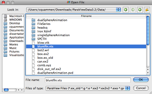
This tutorial assumes that you have not performed any actions before following the tutorial steps. For instructions on how to start ParaView, see section 1.2.2, Starting ParaView. To load the data file you will use in this tutorial, select "File | Open File" from the Menu Bar. This will launch a file selection dialog like the one shown below.
Figure 1. File Open Dialogs
Initially, the file selection dialog shows all files with extensions that ParaView recognizes. You can limit the display to files of certain type by selecting a different filter using the "Files of type:" menu.
Navigate to the folder in which the tutorial data files are located. (The tutorial
data files are available in the Download section of the ParaView web site, here.) Next, select 'bluntfin.vts'
and click the 'Open' button. (If the file is not listed, make sure that the
tutorial data files have been downloaded and extracted and that the file selection
dialog is showing all ParaView file types by selecting ParaView Files in the
"Files of type:" menu.) The left panel of the ParaView window should now look
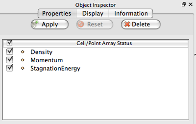
similar to the image shown on the left. Up to this point, ParaView read information
about the contents of the data file but did not actually read any data. This
allows the user to change certain properties of the reader before the file is
read. As shown in the picture, the properties frame now contains a list of all
the data arrays (variables, attributes) available in the file. In this case,
the file contains two scalar variables called Density and StagnationEnergy and
one vector variable called Momentum. By default, all arrays are selected and
will be read if you click the 'Apply' button. However, since you will need only
the Momentum vector in this tutorial, you can reduce the load time and memory
consumption by deselecting the Density and StagnationEnergy scalars. Note that
only some readers support this feature. If a reader does not have any properties
accessible to the user, it will immediately load the data file. After deselecting
Density and StagnationEnergy, click 'Apply'. The ParaView window should now
resemble the image below.
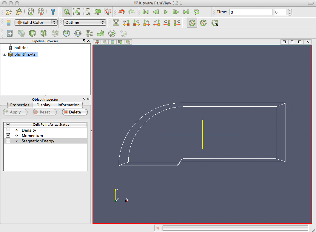
Figure 2. ParaView window after opening a structured grid data file.
The file you just loaded contains structured grid data showing the supersonic flow over a flat plate with a blunt fin rising from the plate. It was converted from a PLOT3D file distributed by NASA. You will notice that only a wireframe outline of the grid is displayed. ParaView displays structured datasets (rectilinear and curvilinear grid) and large unstructured grids as outlines and polygonal data and small unstructured grids as surfaces. For more information on data types supported by ParaView, see section 2.3 of the User's Guide.
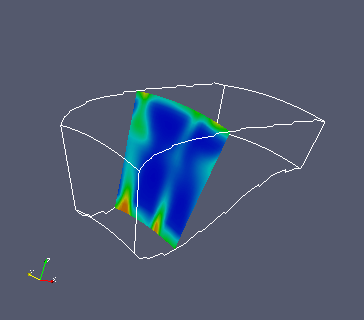
Next, we will extract two 2D sub-grids from the structured grid using the extract filter. Click on the 'Extract Subset' icon on toolbar or use Filters/Alphabetical/Extract Subset to create the first filter. In the VOI (Volume of Interest) section of the property sheet shown on the Left Panel, set the minimum and the maximum values of I to 18 by either typing in the entry box or using the sliders (these values are shown in the top row of the VOI table). Click 'Apply'. The output should look like the image below. If you have only an outline wire-frame of the slice, use the Display tab and change the Representation to Surface.
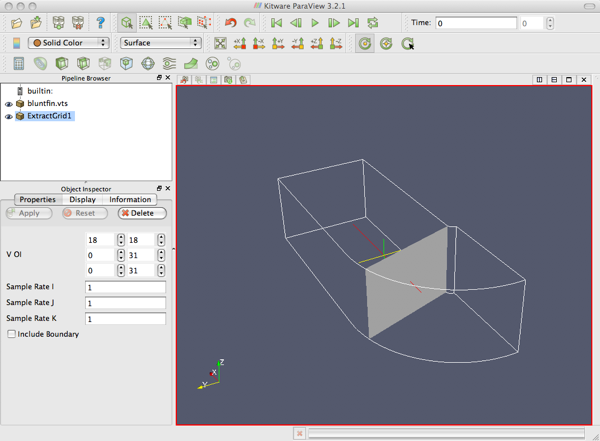
Figure 3. First sub-grid
Extract Subset is a filter that either selects a portion of a structured grid dataset or sub-samples it. The selected portion is referred to as the Volume of Interest (VOI). The sampling rate is determined by the 'Sample Rate' parameters. Note that screen shot above was generated after changing the camera position by using the 3D interaction afforded by the mouse (left-click-and-drag rotates, middle-click-and-drag pans, right-click-and-drag zooms in/out. To change the color mapping of the new plane, select the Display page and choose 'Momentum' from the 'Color By' menu. The current version of ParaView uses a blue-gray-red colormap by default rather than the rainbow (thanks to a paper written by a student after taking this class), so the color will look different from the image below.
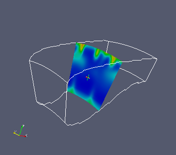
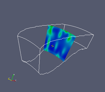
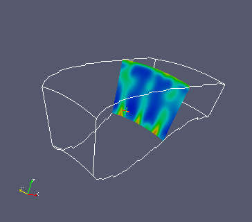
Next, we will extract the fin surface. First, make sure that the 3D structured grid is the active data. (Click on 'bluntfin.vts' in the Pipeline Browser.) Now create another extract filter by clicking on its icon on the toolbar. Set the minimum and the maximum of J (second row in the VOI section) to 0 by either typing in the entry box or using the spinners. Click 'Apply'. ParaView should now look like this.
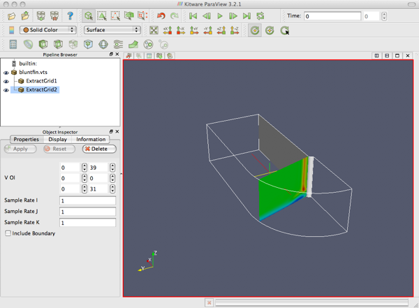
Figure 4. Second sub-grid.
Next, we will add some streamlines. First, make sure that the 3D structured grid is the active data. (Click on 'bluntfin.vts' in the Pipeline Browser.) Then, create a Stream Tracer filter by clicking on the 'Stream Tracer' icon on the toolbar (or using Filters/Alphabetical/Stream Tracer). The Stream Tracer filter has more complicated properties than previously encountered. There are two sections on the Properties page. The first one allows you to modify the integrator properties of the Stream Tracer filter. The second one, Seeds, allows you to specify the creation of seed points of a streamline (the starting point of a particle as it is advected through the vector field). In the display window, a 3D widget that allows interactive adjustment of the seed points is shown by default. To better see the widget, you can turn off the visibility of the first sub-grid by clicking on the eye icon next to ExtractSubset1 in the Pipeline Browser.
|
|
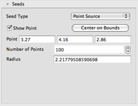
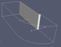
| The property page component of the seed parameter. | The 3D widget component of Line Source seed is shown in the foreground. |
ParaView supports a few manipulators (3D widgets) to allow users to easily change parameters. For a list of the 3D widgets used in ParaView, see Appendix A in the User's Guide. You will first use a line to seed the streamlines. Under the Seeds section of the Properties page, select Line Source as the seed type from the pull-down menu labeled Seed Type. Next, set point 1 to (-3.59, 0.33, 2.86) and point 2 to (-3.59, 5.48, 2.86) by typing in the entry boxes. You can also change the position of the end points by clicking on the spheres at each end of the line shown in the display window and dragging. Then, set the Resolution to 10. Finally, under the Stream Tracer section, set the Maximum Streamline Length to 10 and set the integration Direction to FORWARD. Click Apply. The output should look like the following.
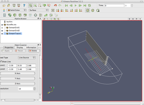
Figure 6. Streamlines created with a line source.
Next, we will move the seed to a more interesting region. First, change the seed type to Point Source, and change the Radius to 0.3 and the Number of Points to 10. Next, position the center of the point cloud at approximately (-0.54, 0.28, 0.55) by typing in the entry boxes. (You can also move the point widget by clicking on one of the axes and dragging.) This point is near the stagnation point on the plate-fin juncture. Click Apply. The Point Source will create 10 points randomly placed in a sphere of radius 0.3 centered at the position of the point widget. To view the structure in the juncture region more closely, move the camera near the center of the point cloud.
Unshaded polylines are not the best way to visualize streamlines in 3D. Adding some thickness (and shading) can make it much easier to comprehend the three-dimensional structure of the flow field. This can be done by using either the Tube or the Ribbon filter. The tube filter generates tubes around input lines, whereas the ribbon filter generates oriented ribbons from the input lines. In this tutorial, we will use the tube filter. First, make sure that the streamline filter's output is the active data. (Click on StreamTracer1 in the Pipeline Browser.) Next, create a tube filter by selecting Filters/Alphabetical/Tube. Set the Number of Sides parameter to 8 and Radius to 0.03. Click Apply. You can change the color mapping by selecting the Display tab in the Object Inspector and selecting the AngularVelocity from the Color by menu. The ParaView window should now look like this (but with a blue-gray-red colormap).
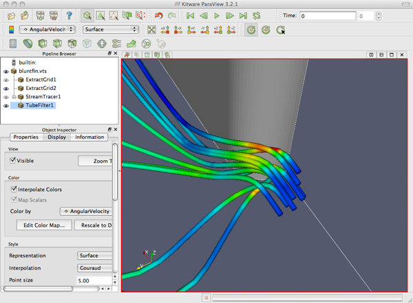
Figure 7. Tubed streamlines.
You might have noticed that the filters available in the Filters menu do not always remain the same. This is because the Filters menu is context sensitive and will only enable filters applicable to the current data object. For example, if the current object is of type structured grid, the tube filter will not be active in the Filters menu since it can be only applied to polylines. Similarly, if the current data object does not contain any three-component vectors, the streamline filter will not be available. Every time a new data object is created or selected, ParaView modifies the availability of the filters in the filter menu by comparing the requirements of each filter to the properties of the current object and adding only applicable filters.
Since the example data file used in this tutorial was small, the streamline calculation took very little time and can be easily repeated without any inconvenience. However, as the data files become larger, such calculations may take a long time. In such cases, it might be useful to store the result of the calculation so that it can be restored later and viewed in 3D. To save the output of the tube filter, select the Tube1 object from the Pipeline Browser and select File/Save Data. This will bring up a Save File selection window that is very similar to the Open File dialog. Change the path to the directory where you want your data file(s) stored. In this case, you can write the data object in five different formats: ParaView Data format (*.pvd), VTK polydata format (*.vtp), PVTK polydata format (*.pvtp), legacy VTK format (*.vtk), PLY Polygonal File Format (*.ply), XDMF format (*.xmf), and comma-separated file (*.csv). This concludes the second tutorial. You can now exit ParaView by either selecting File | Exit or closing the window.
This tutorial will introduce ParaView's animation interface. It will demonstrate the use of a few ParaView filters, including the isosurface, clip, and cut filters, and show how these can be controlled by the animation editor. If you are not familiar with ParaView, we recommend that you read the first tutorial before working through this example.
This tutorial assumes that you have not performed any actions before following the tutorial steps (so quit and re-start ParaView). Otherwise, the names of the modules created might vary. For instructions on how to start ParaView, see section 1.2.2 of the ParaView User's Guide.
In this example, we will use a PLOT3D file. The PLOT3D format stores the geometry (structured grid) and the attributes in separate files. First, open the geometry file by selecting File/Open, navigating to the folder in which the tutorial data files are located, choosing comb.xyz in the file selection dialog, and clicking the Open button; then select PLOT3D as the reader to use to open this file. (The tutorial data files are available in the Download section of the ParaView web site.) You should now see the parameters page for a new PLOT3D reader.
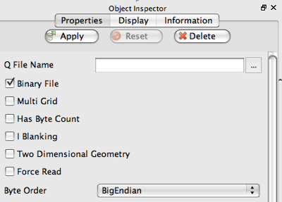
Figure 8. PLOT3D reader parameters.
Click Apply. Double-click on the comb.xyz file in the Pipeline Browser and change the name to Combustor Data. (Make sure you press Enter after typing the new label; otherwise the change will not take effect.) By assigning more meaningful labels, you can make finding a module in the Pipeline Browswer much easier, especially when there are many modules.
Once the file is loaded, certain buttons in the toolbar will be enabled while others remain disabled. This is because, like the filter menu, the toolbar buttons are context sensitive. So far, you have only loaded the geometry file. The data object that was created does not contain any data arrays (scalars, vectors, etc.). Therefore filters that require data arrays, like Array Calculator, Warp, Threshold, and Contour, are disabled. To load the attributes, click on the '...' button next to the Q File Name parameter (you may need to scroll down to see it), select comb.q in the file selection dialog, and click Open. Click Apply to load the attributes file. Notice that all the toolbar buttons are now enabled.
Next, we will extract a density isosurface by using the contour filter. You can either use the contour button on the toolbar or choose Filters/Alphabetical/Contour to create a contour filter. By default, the contour filter is created with a single contour value shown in the Isosurfaces section. The Property page should now look like this:
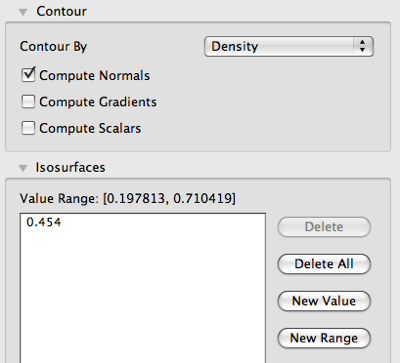
Figure 9. Contour Properties page.
Here, the Contour By menu allows the user to choose which data array to use in creating the isosurface. Any one-component, or scalar, array can be used to create isosurfaces. If you click on the Contour By menu, you can see that the available arrays are Density and StagnationEnergy. Next, the range of the currently selected array is shown. You can add isosurface values by using the Add Value button or the New Range button. To change a value in the list of contour values, double-click on a value. To remove a value from the list, select it and click Delete. All of the contour values can be removed from the list by clicking Delete All. Start by modifying the default isovalue to 0.3 by double-clicking it. Make sure the Compute Scalars box is checked. Next, click Apply. Then, change the name of the contour filter in the Pipeline Browser to Animated Contour. The ParaView window should now look like this.
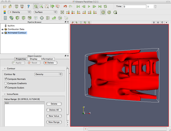
Figure 10. First contour.
Because the isosurface displayed covers a large portion of the whole grid, it is difficult to see some of the details at the center of the domain. You can remove part of the isosurface by using the clip filter. First make sure the contour filter (Animated Contour) is selected. Create a clip filter by either clicking on the Clip button on the toolbar or by selecting Filters/Alphabetical/Clip. The default clipping surface is a plane. The orientation and center of the plane can be modified by either interacting with the 3D widget in the display area or changing the values in the appropriate entry boxes. See Appendix A in the User's Guide for the descriptions of the most common 3D widgets. In this example, the default parameters of the plane are good. Click Apply. You will notice that the clipped iso-surface replaces the whole iso-surface. This is because when a clip filter is created, the visibility of its input is automatically turned off by ParaView. Change the label of the clip filter to Clipped Contour. Next, change the color mapping of the surface by selecting the Display tab and changing Color by to Momentum. To color by the x-component of the Momentum vector, Magnitude pull-down, and select X. The ParaView window should now look like this (but without the rainbow color).
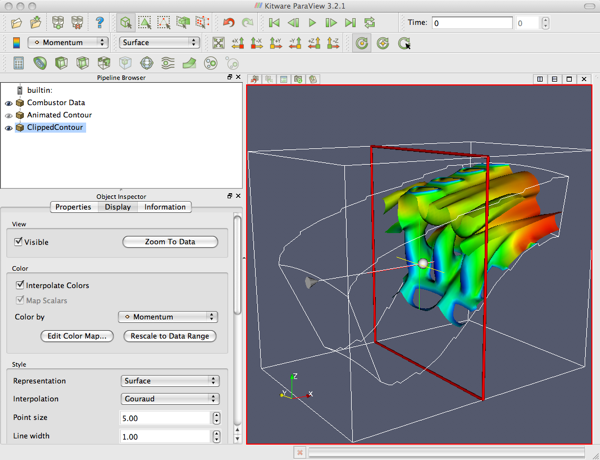
Figure 11. Clipped contour (colored by the x-component of Momentum).
You can turn off the visibility of the plane widget by going back to the Properties page and disabling the Show Plane checkbox.
In this section, we will demonstrate how to create an animation that sweeps over a range of isosurface values by using ParaView's animation editor. First, make the Clipped Contour invisible by clicking on the eye icon next to the item in the Pipeline Browser. Then, color the Animated Contour by the x-component of Momentum (after making it visible by clicking on the eye next to it). To display the animation editor, select View/Animation View. A new panel should appear below the display window as shown below.
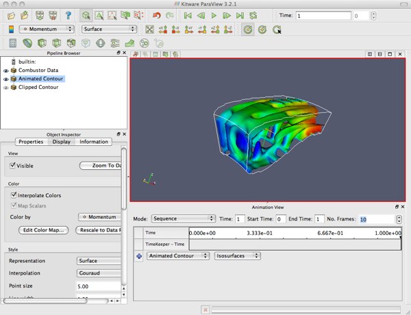
Figure 12. Animation viewer interface.
Change the No. Frames parameter to 50. Make sure the Animated Contour is selected in the menu to the right of the plus sign, and click on the plus sign. A new row in the table will show up above the row with the plus sign. Double-click somewhere on this row. A window will appear with a table consisting of three columns: Time, Interpolation, and Value. The Time column shows the time when the isosurface value will be the value under the Value column. The Interpolation column controls how the values are interpolated between keyframes. Set the value at time 0 to 0.3 and at time 1 to 0.6 and click 'OK'. The Animation Viewer should now appear as shown below.
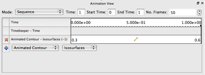
Figure 13. Animation viewer prior to animation.
The middle part of the top tool bar contains controls for animation. The control buttons work similarly to a VCR - they do the following things, in order from left to right: return to the beginning of the animation, move one frame back in time, play the animation, advance one frame in time, jump to the last frame of the animation, and toggle looping of the animation. Play the animation.
To save the animation, choose the File/Save Animation menu item. The animation may be saved as an AVI file (on Windows) or as a sequence of numbered image files.
Before moving to another animation, we will demonstrate how to delete existing ParaView modules. First, select the Animated Contour object in the Pipeline Browser and select the Properties tab. You will notice that the Delete button is disabled. This is because the output of the contour filter is used by the clip filter. ParaView does not allow the deletion of a module if its output is used by another module. To delete the contour filter, first select the clip filter (Clipped Contour), delete it, and then delete the contour filter. It is also possible to delete all modules by selecting Edit/Delete All. However, since we will need the reader module in this example, do not use this.
In this section, you will create a cut-plane through the combustor dataset and move it in an animation. Create a slice filter by either clicking on the Slice button on the toolbar or selecting Filters/Alphabetical/Slice. Change the label to Cut-plane, turn off the visibility of the 3D widget by clicking on Show Plane in the Properties page, and accept all other default parameters by clicking Apply. The ParaView window should look like this (with a blue-gray-red colormap).
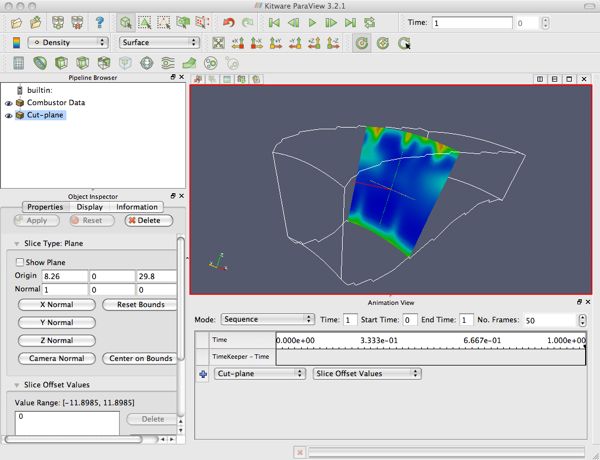
Figure 14. Cut-plane to be animated.
Next, take a look at the Animation View. Delete the previous animation action for the Animated Contour using the red X. Add a new action by selecting Cut-plane as the source and clicking the plus sign. Set Slice Offset Values as the parameter, -5 as the value at time 0, and 5 as the value at time 1. Change No. Frames to 20 and play the animation. The Animation View should look as shown below.
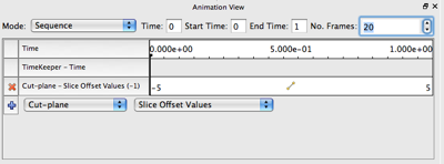
Figure 15. Animation View prior to animating the cut-plane.
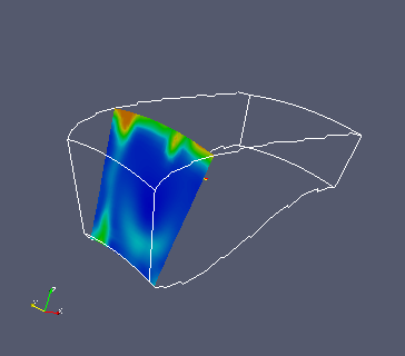 Frame 0 |
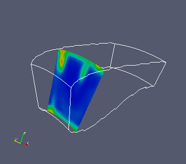 Frame 2 |
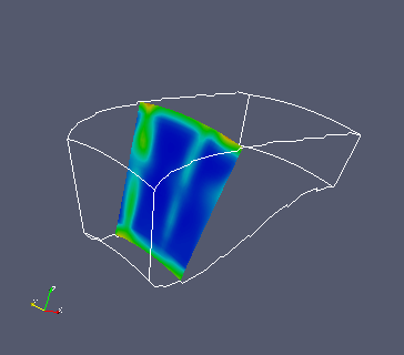 Frame 4 |
 Frame 6 |
 Frame 8 |
 Frame 10 |
 Frame 12 |
 Frame 14 |