Kecheng Yang (yangk@cs.unc.edu)

Assignment 2 Part II

2(II).Graph Cuts

---

2(II).1 Description and requirements

Now we will add a component using graph cuts to find the region of an image to insert into another image instead of doing this by hand. You will need to find code to do graph cuts in Matlab---in particular we are looking for min-cut, max-flow algorithms that minimize the sum of weights of edges that are cut to separate a source and a sync. There are many version of this type of code available. You can exchange ideas about good sources for this code on the Sakai site for the class. You will then have to formulate the problem of finding a good region as a graph-cut problem. This will involve defining the graph based on the image(s) involved, passing it to the graph-cut algorithm, and interpreting the result to automatically crop out a region. Then you will use the first part of your assignment to blend this region into an image.

You should also collect a set of at least 50 images with similar content and search through these to find one for use in the assignment.

---

2(II).2 Max-flow/Min-cut

Use max-flow/min-cut to find the region of the image to insert to another one.

I used the maxflow code from http://www.math.ucla.edu/~wittman/Fields/maxflow.zip

The usage format is "[flow,labels] = maxflow(A,T);".

---

2(II).3 Construct the graph

We need to construct the graph for the maxflow algorithm, and I constructed the graph following the instructions in the slides of lecture8.

For the initial setting, I set the four outside edges of the figure to be background and use imfreehand() to specify the a small area that is definitely in foreground. Also, initial unary is set great enough.

The code is:

m = double(rgb2gray(im));
[height,width] = size(m);

disp('building graph');
N = height*width;

unary = 9e9;

% construct graph
E = edges4connected(height,width);
figdis = gmdistribution.fit(m(:),1);
V = exp(-((m(E(:,1))-m(E(:,2))).^2)/(2*figdis.Sigma*figdis.Sigma));
A = sparse(E(:,1),E(:,2),V,N,N,4*N);

T = sparse(N,2);

for y = 1:height
    for x = 1:width
        if y==1 || y==height || x==1 || x==height
            T((x-1)*height+y,1)=unary;
        end
        
        if front(y,x)
            T((x-1)*height+y,2)=unary;
        end
    end
end

---

2(II).4 Iterations

In this part, we use the labels got in last maxflow() to re-define background and foreground. Also, use Gaussian Mixture Model to re-compute unary for each node.

Do the iterations until labels does not change anymore.

The code is:

while sum(labels(:)) ~= sum(old_labels(:))
    count = count + 1;
    fi = find(labels(:)==1);
    bi = find(labels(:)==0);
    fg = m(fi);
    bg = m(bi);
    fgdis = gmdistribution.fit(fg,1);
    bgdis = gmdistribution.fit(bg,1);
    
    tmp = m(:);
    unary_v = -log(fgdis.pdf(tmp)./bgdis.pdf(tmp));
    unary_b = unary_v;
    unary_v = abs(unary_v);
    pos = find(unary_b >= 0);
    neg = find(unary_b < 0);
    unary_b(pos) = 1;
    unary_b(neg) = 2;
    
    i(1:N,1)=[1:N];
    v(1:N,1)=unary_v;
    j(1:N,1)=unary_b;
    T = sparse(i,j,v,N,2);
    old_labels = labels;
    [flow,labels] = maxflow(A,T);
    labels = reshape(labels,[height width]);
end

The code for getting the region by using graph cut is mygraphcut.m.

---

2(II).5 Result

Now, we use labels as bMask in part I of this assignment, then we can use techniques in part I to blending images.

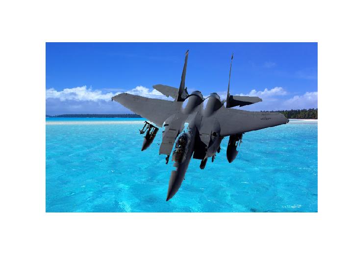
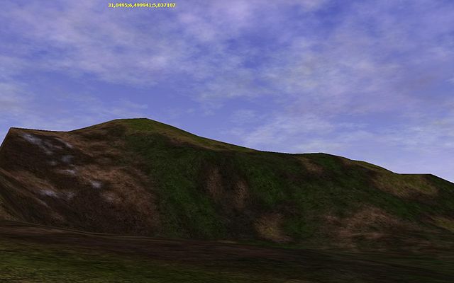
The sources and the target are as follows:

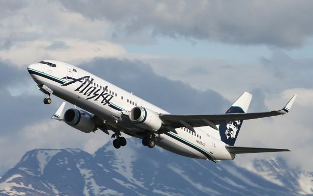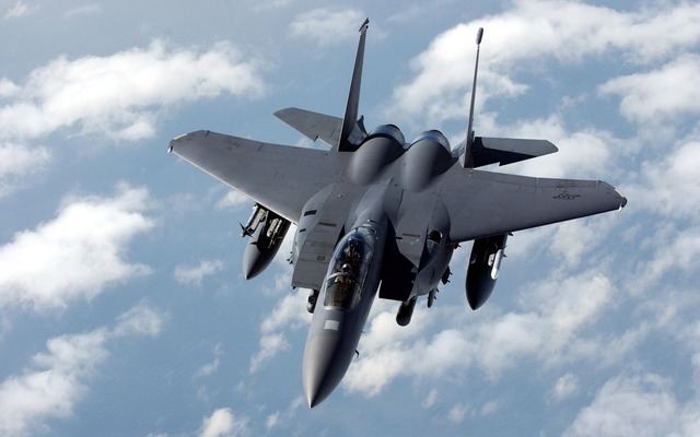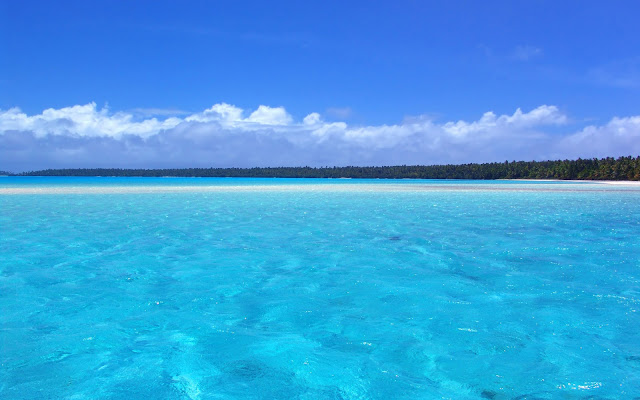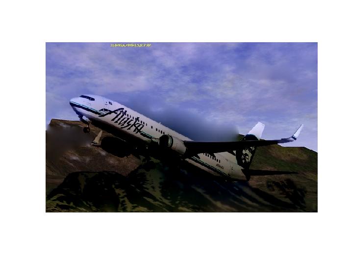
The result is as follows:

---

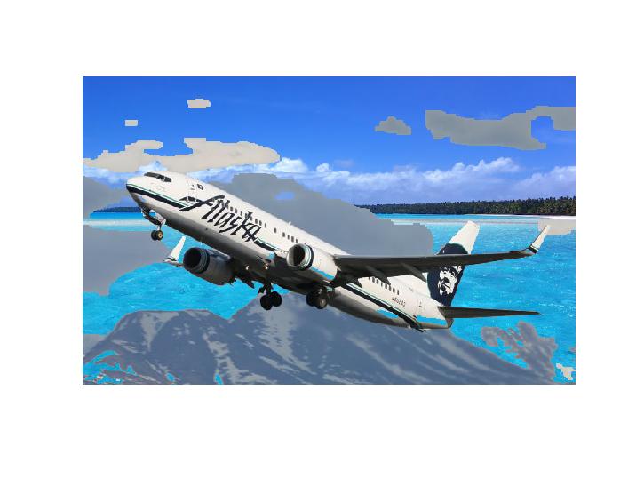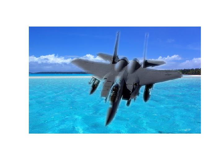2(II).6 COMP 790 additional part

Now we collect a set of 50 images, and use GIST as the criteria to select one as background to best fit our sources.

The core part of the code is:

for index=1:50

    target_name=sprintf('targets/target%d.jpg',index);
    img2 = imread(target_name);

    % Parameters:
    clear param 

    param.orientationsPerScale = [8 8 8 8];
    param.numberBlocks = 4;
    param.fc_prefilt = 4;


    [gist2, param] = LMgist(img2, '', param);


    gist_diff(index) = sum((gist1-gist2).^2);
end

Then we use [mini_v mini_index] = min(gist_diff) to find the best-fit backgound index.

The code for computing gist_diff is selectbg.m.

---

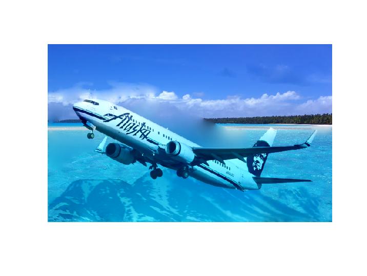
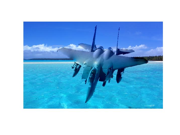
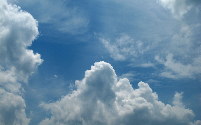
2(II).7 Best-fit background blending

We use GIST to search for the best background. For the two sources, we got different best back grounds.

The 50 candidate images are provided here.

The following are the final result. Note that we use gradient domain blending.

---
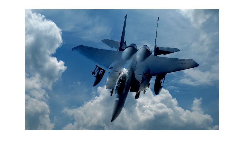