Assignment 5
5. Free-Choice Assignment: average image of non-fixed position photo samples
5.1 Description and requirements
This is an assignment of free choice. Motivated by the lecture of average images, I decided to do an average image of a landmark object.
In the lecture, we assumed the camera is fixed in one position all the time to take a bunch of photographs, and then calculate the average value of each pixels. By this way, the temporary object in a small part of those photos, e.g., moving pedestrians or cars, will be non-noticeable in the resulting average image.
In this assignment, I consider to make the average image for a set of photos of a same object where the position of the camera that took the photos may vary, the sizes or shapes of the photos may not be consistent, and/or the light on the object may also slightly change. I leverage the correspondence techniques from the assignment for panoramas to align all the samples up.
Furthermore, I also explore different ways other than average value to make the "average" image.
5.2 Example object and samples
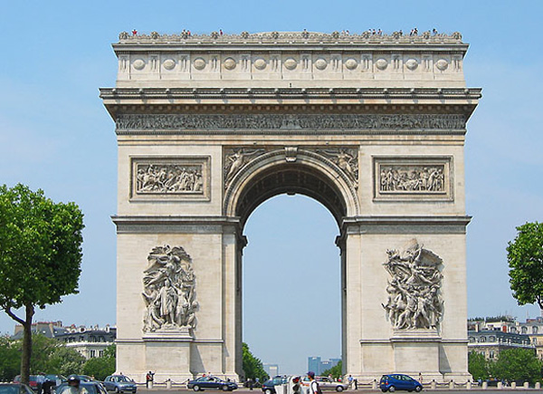
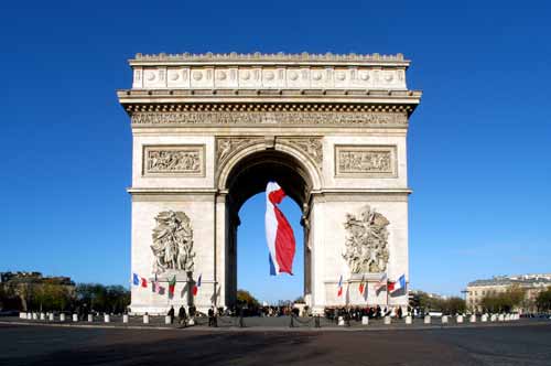
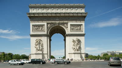
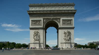
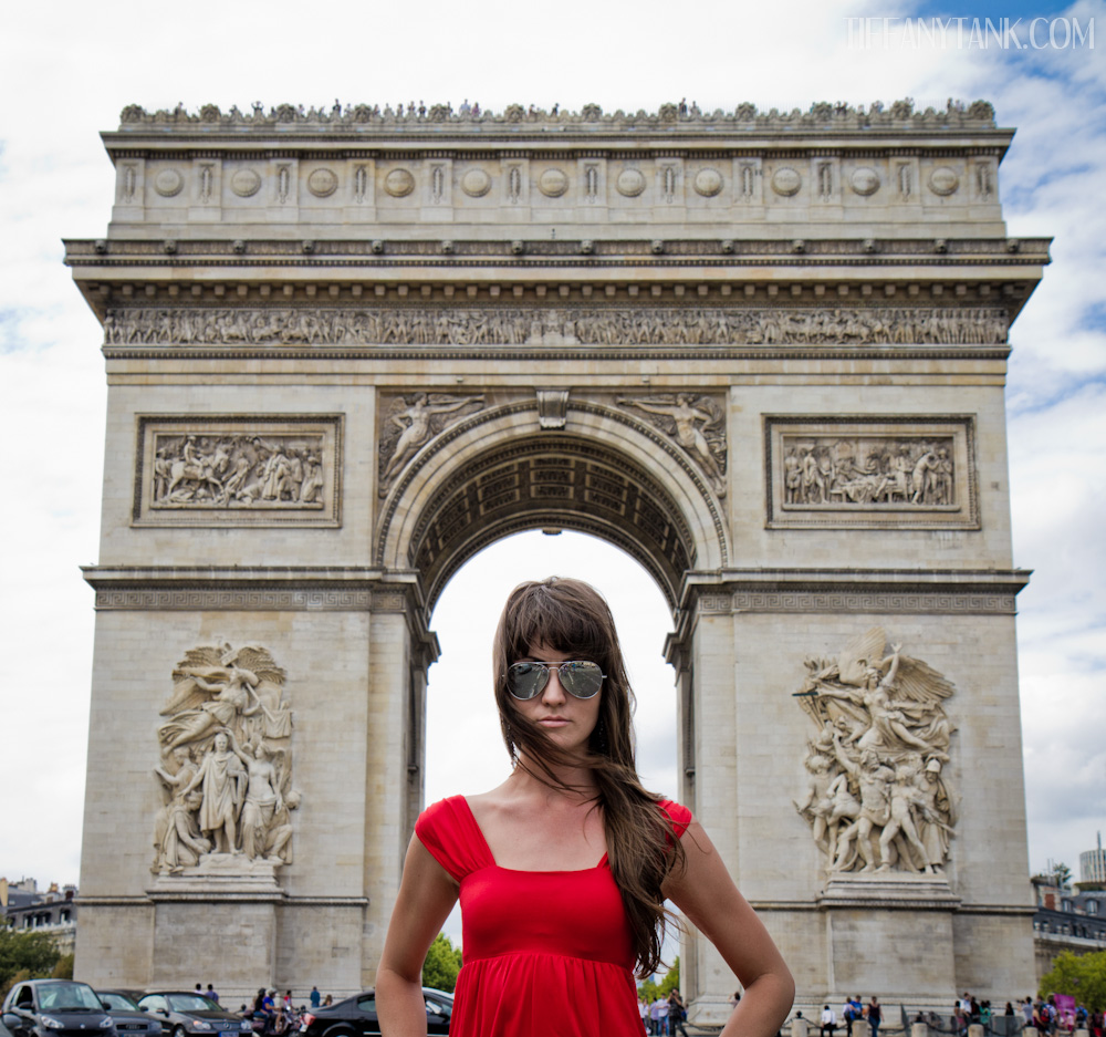
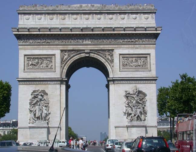
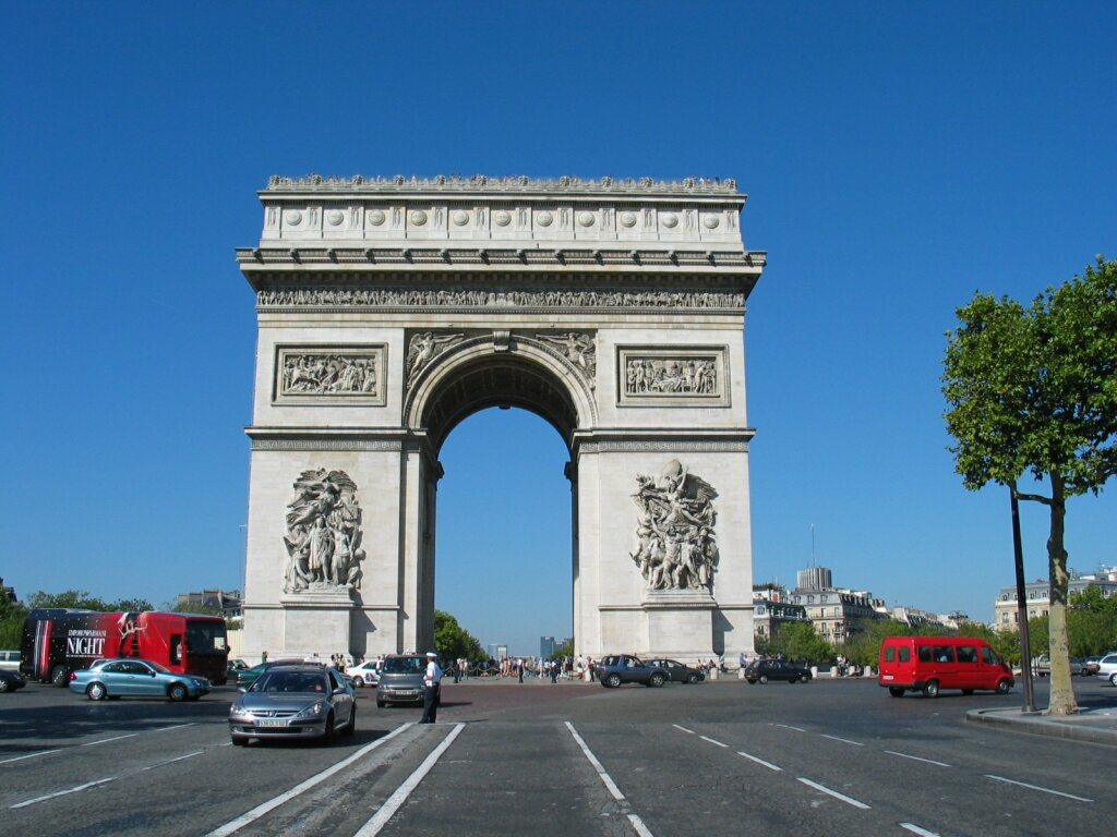
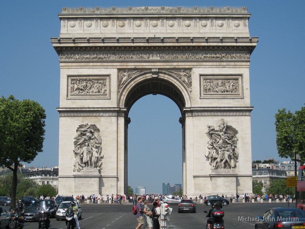
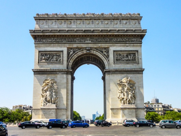
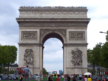
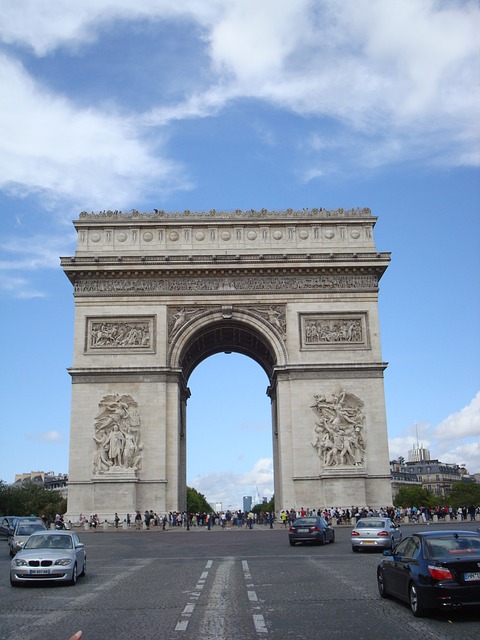
In this assignment, I chose Arc de Triomphe as the landmark to illustrate the method, because it is a unique landmark with a lot of features (also because I was there during a conference last October ^_^).
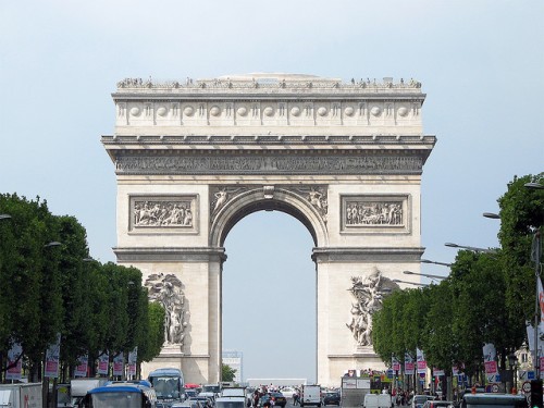
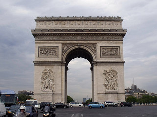
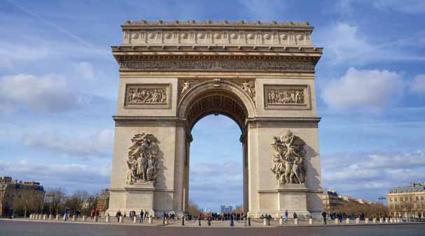
The following images are well front-view Arc de Triomphe photos which I got from Google Images.
For the purpose of shortening the computation time, I only gatherer 16 photo samples, and each of them is not of huge resolution (generally less than 1000*1000).
 |  |  |  |
 |  |  |  |
 |  |  |  |
 |  |  |  |
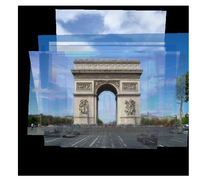
5.3 Align the samples
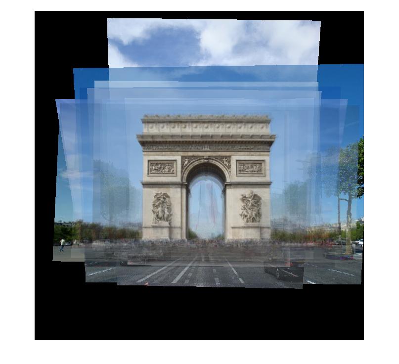
As we can see, among these samples above, the camera is not fixed in a single place, and the light also varies. Moreover, the shapes and resolutions of those photos are not identical either. Therefore, we cannot simply do the math to compute the average value of each pixel to get the average image. To deal with this problem, I apply the techniques in last assignment, panoramas, to find feature correspondences between photographs, and then compute the homograph matrix by the correspondences. Finally, I transform the photographs via the homograph matrices to align all the samples.
Specifically, I use the sample 0 as the template. I move it to the center of a 1000*1000 pixels empty image, and use this as the standard position. Then transform all other samples to be aligned to sample 0 in a 1000*1000 empty background also. Now we can compute the average images for these aligned samples.
The code for this is just slightly modified from the code for the automatic correspondence with RANSAC in last assignment.
5.4 Compute the average image
When we talk about "average" image, it may not be just the average values of each pixel. In this assignment, I explore several different way to derive the "average" image.
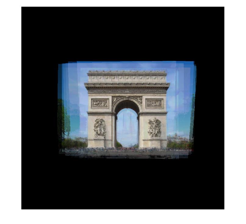
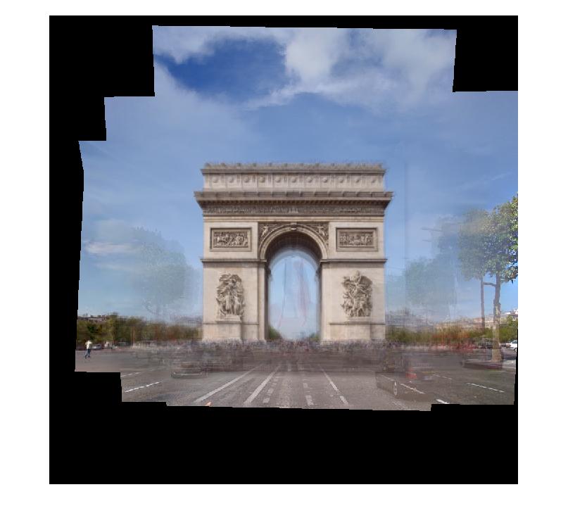
5.4.1 Average values
The most intuitive way to compute the "average" image is to compute the average value for each pixel. One of the tricky thing is that not all pixels in our aligned samples are significant. Those outside zeros may only mean "invalid" pixel. If we do not consider this, then we will get much lighter colors in non-center part of the resulting image, since those pixels are the average of the valid ones and some zeros. Thus, I compute how many valid values we should account for at each pixel, then compute the average of all valid values. The code is following.
samples = zeros(result_imw,result_imh,3,N+1);

...

masks = (samples>0);
masks = double(masks);

total = sum(samples,4);
valid_pixel_nb = sum(masks,4);
average_im = total./ valid_pixel_nb;
average_im(isnan(average_im))=0;

average_im = uint8(average_im);
The result is:
5.4.2 Medians
Another statistical parameter we could consider is the median. I use the median across samples for each pixel as the value of this pixel
via the simple code "simple_median = median(samples,4);". Then I get the following result. The reason why only center part have
non-zero value is that if at a pixel, more than half the sample is just 0, then it is obvious that the median is 0 too.
5.4.3 Medians of valid values
Similar to the average-value method, we can also only consider valid pixel values with respect to medians. The relevant code is:
precise_median = zeros(result_imh,result_imw,3);
for color = 1:3
    for y=1 : result_imh
        for x = 1:result_imw
            clear valid_values;
            valid_values = samples(y,x,color,samples(y,x,color,:)>0);
            precise_median(y,x,color) = median(valid_values);
        end
    end
end
precise_median(isnan(precise_median)) = 0;
precise_median = uint8(precise_median);
The result is:
5.4.3 Average gradient
In any of the above three methods, one most noticeable thing is that the borders of overlapped samples are not removed in the average image, and that makes all the non-center parts image ugly.
To remove those overlapping borders, we consider to process the image in gradient domain.
From the "toy program" of assignment 2, I learned that given the value of one pixel, and gradients of all pixels, we can recover or reconstruct the whole image. Therefore, my strategy in this assignment is that use the average value of the very center pixel, i.e. (500,500) in this example, as the value of the center pixel in the result. In addition, I use the average gradient at all pixels as the gradient at corresponding pixels in the result. Then we can get the result by solving linear equations.
Note that when we compute the average gradient for a pixel, we also only consider valid ones among the samples. If at some pixel, every sample is invalid, i.e. 0, then we do not consider gradient at this pixel in the result, we just set it equals to 0.
The main part of the code is:
direction = 4;

gradient = NaN(imh,imw,direction,3,N+1); %direction: 1-up,2-down,3-left,4-right

masks = (samples>0);

for sample_num = 1:N+1
    for color = 1:3
        for x=1:imw
            for y=1:imh
                if masks(y,x,color,sample_num)
                    if y > 1 && masks(y-1,x,color,sample_num)
                        gradient(y,x,1,color,sample_num) = samples(y,x,color,sample_num)-...
                            samples(y-1,x,color,sample_num);
                    end
                    if y < imh && masks(y+1,x,color,sample_num)
                        gradient(y,x,2,color,sample_num) = samples(y,x,color,sample_num)-...
                            samples(y+1,x,color,sample_num);
                    end
                    if x > 1 && masks(y,x-1,color,sample_num)
                        gradient(y,x,3,color,sample_num) = samples(y,x,color,sample_num)-...
                            samples(y,x-1,color,sample_num);
                    end
                    if x < imw && masks(y,x+1,color,sample_num)
                        gradient(y,x,4,color,sample_num) = samples(y,x,color,sample_num)-...
                            samples(y,x+1,color,sample_num);
                    end
                end
            end
        end
    end
end

gradient_masks = not(isnan(gradient));
valid_gradient = any(gradient_masks,5);
valid_point = any(valid_gradient,3);

gradient_masks = double(gradient_masks);
gradient(isnan(gradient)) = 0;
total_gradient_masks = sum(gradient_masks,5);
total_gradient = sum(gradient,5);

average_gradient = total_gradient./total_gradient_masks;
5.5 Discussion
In the results, we find the temporary objects, e.g. the woman and the flag, may not be totally removed. Looking carefully, we can see the shadows of them in the results. I think it is probably because of the limited sample number, which is 16. I believe if we use 50 samples or 100 samples or even more, then the result would be even much better. The reason why I did not do so is that finding suitable samples is kind of time consuming. Also, more samples means more computation time, which might make the program even more time consuming. As I think current result has clearly shown the points I wanted to show for this assignment, I decided not to increase the number of samples.
Moreover, when I did this assignment for the first time, some of the samples were transformed to nonsense images. I believe it is because in those samples, the light or the depth or the angle of the camera might vary too much from our standard one, sample_0, and therefore the computed homograph matrix is incorrect or even invalid. In this assignment, I just manually tested and aborted such samples.
I would suggest an advanced step for this assignment to be that making an automatic program to retrieve and select "good" samples, which might even involve some machine learning related work. Due to the limited time and my limited image processing or machine learning experience, I would consider this advanced step is beyond the scope of this assignment.
5.6 Source
The workspace of this assignment is packed as photog_a5.zip, including all codes and sample photographs.
Please run auto_align_samples first, then run avg_gradient.
The resulting images are average_im, simple_median, precise_median,
and output, respectively.