Assignment Summary

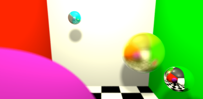
    This assignment explores different visual effects that are possible with a distributed ray tracer; supports soft shadows from area lights, depth of field, and blurred reflections.

The Code:  (Download)

    In this assignment I extended my Whitted ray tracer from Assignment 1 to become a distributed ray tracer.  I continued to use Peter Shirley’s book “Realistic Ray Tracing” as a guide through the process.  However, these new features required extra clarification for me, so I also studied some of the materials that Shirley references in his book in addition to class slides.

    New features in the ray tracer:

1. ‣Soft Shadows:  Illumination provided by spherical luminaires.
   

2. ‣Depth of Field:  Depth of field is implemented using the thin lens model.
   

3. ‣Blurred Reflection:  Implemented using a Phong-like model to determine reflection ray distribution.
   

4. ‣Diffuse-Specular Materials:  In support of blurred reflection, I added support for diffuse materials with specular components.  Diffuse/Specular components are balanced with approximated Fresnel equations.

Soft Shadows

    Soft shadows may be implemented by using an area light.  At illumination time, multiple shadow rays are cast back towards the surface of the area light to sample visibility of the light’s surface.  Portions of the area light are partially obscured at views along a shadow’s edge.  Thus, edges appear soft when the distributed rays are averaged together.

    My ray tracer uses a spherical area light (luminaires) to provide lighting.  Shirley describes a technique for sampling the surface of the sphere in his book (and several more in his papers).  Here is the book’s technique described without the mathematical details (repeat for each luminaire):

1. ‣Step 1:  Generate samples on a unit disk and scale the disk to the radius of the luminaire.  Traditional unit-square samplers may be concentrically mapped to the unit disk.  There are several different methods to perform this mapping-- area preserving vs. non.  I chose to implement non-area preserving sampling (it’s easy).  This unduly gives extra weight to samples along the disk’s edge (when samples are averaged), but results below still appear to be good.  Please see Shirley’s book, page 103 for concentric mapping algorithm.
   

2.     Aside: Some sampling methods that work well in Cartesian space do not work well when mapped concentrically.  Specifically, Halton sampling.  See results below.
   

3. ‣Step 2:  Compute a ray from the intersection of the surface to be lit towards the center of the luminaire.
   

4. ‣Step 3:  From the perfect surface-to-light ray, construct a basis frame.
   

5. ‣Step 4:  Using the basis frame, transform the sample disk, into global coordinates, to lie within the luminaire.  The disk forms a cross-section along the luminaire’s greater circle, perpendicular to the surface-to-light ray.
   

6. ‣Step 5:  Cast a shadow ray to each sample point on the disk, and average the illumination results.  Note that the disk points have not been mapped to the surface of the sphere.  This distorts results somewhat, though any ray intersecting the surface of the sphere will also intersect the perpendicular greater circle cross-section.  Since my sample points are randomly distributed (jittered n-rook), this distortion has not been a large concern to me.  This issue may need to be revisited if (1) I decided to use a uniform sampling method, or (2) implemented non-uniformly lit luminaries.

Soft Shadow Results

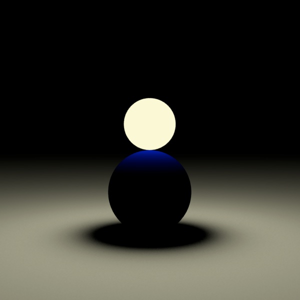
    Below are soft shadow renderings with visible luminaires.  Visibility is not required, but helps show where the lights are located.  Also, pixels were sampled 10 times with jittered n-rook and 20 shadow rays cast per illumination (unless otherwise stated).  Images presented have not been resized.

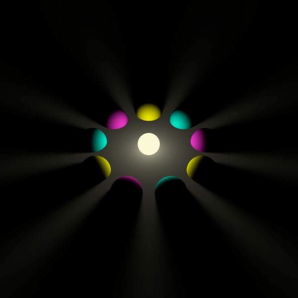
A campfire.

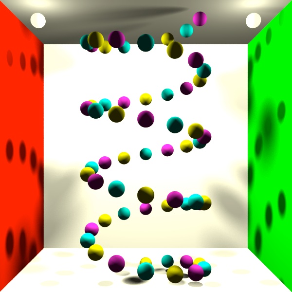
A helix lit with two luminaires.  Shadows from objects farther away from the wall are softer.

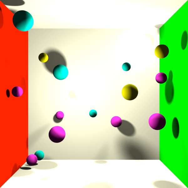
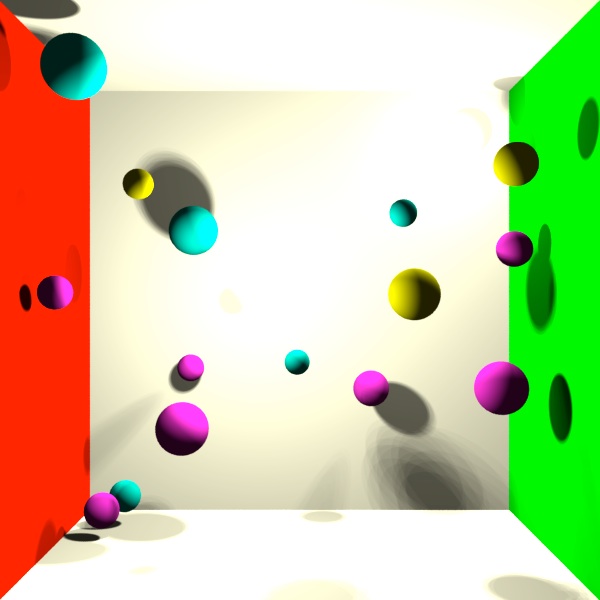
Room with random spheres lit with two luminaires (near center and top right corner).  This image shows a good mix of close (sharp) and distant (very soft) shadows.

Same as previous scene, but with concentrically mapped Halton sampling.

Notice the patterns in the shadows in the lower right corner.

Patterns can be observed on all shadow edges.

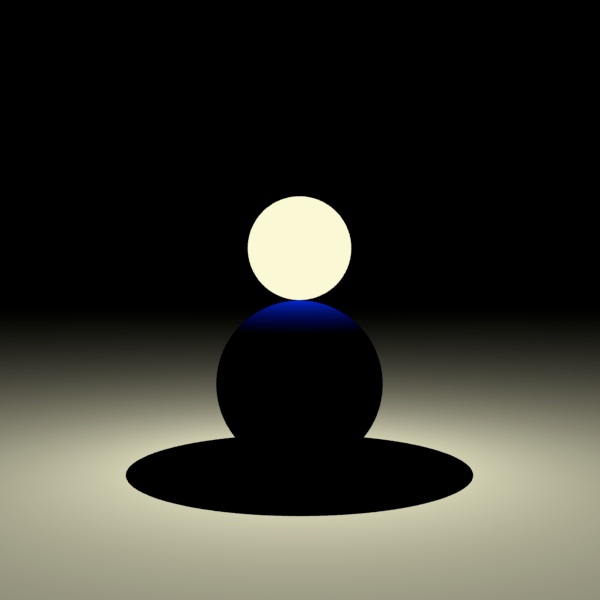
1 shadow ray cast directly to the center of the luminaire.  Essentially a point-light.

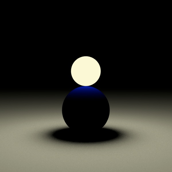
8 shadow rays cast.  Notice noisy shadow edges.

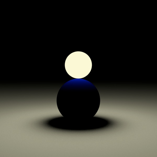
16 shadow rays cast.  Less noise.

32 shadows ray cast per illumination.  Even less noise.  There was no observable difference between this and 62 shadow rays (not shown).

An alternative to averaging distributed shadow rays is to cast 1 shadow ray per pixel sample, but bump up the number of samples per pixel; this method keeps the ray tree “narrow.”  Above is this method with 90 rays per pixel.  This is equal to the number of total rays cast in the 8 shadow ray example earlier (90 = 10 + 8*10).  This method appears to yield more noise.  However, this may be implementation dependent-- my code does not maintain luminaire sampling state between samples within the same pixel.  This makes it impossible to insure a good sample discrepancy of the luminaire surface area.  This limitation could be overcome with some code rework.

Depth of Field >