Splines, Aliasing, and Principal Components
Kyle Moore
COMP 665 - Images, Graphics, Vision
Professor Gary Bishop
November 20, 2006
Part 1
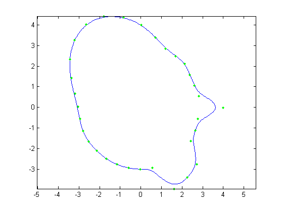
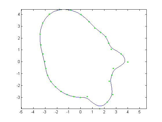
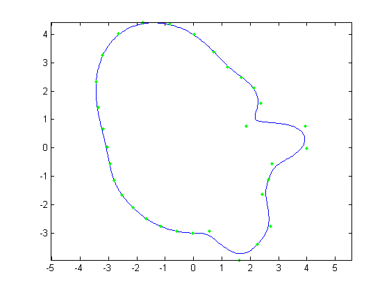
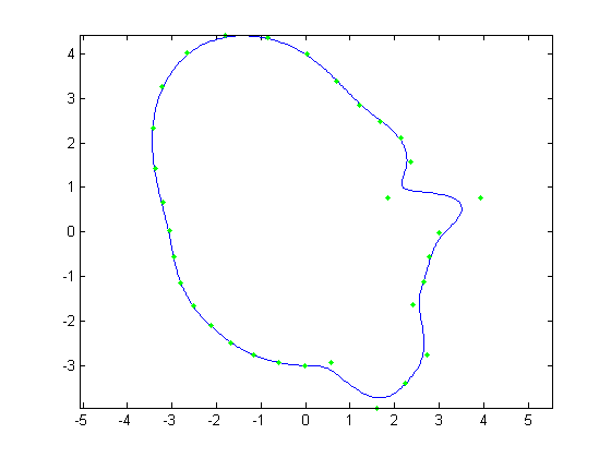
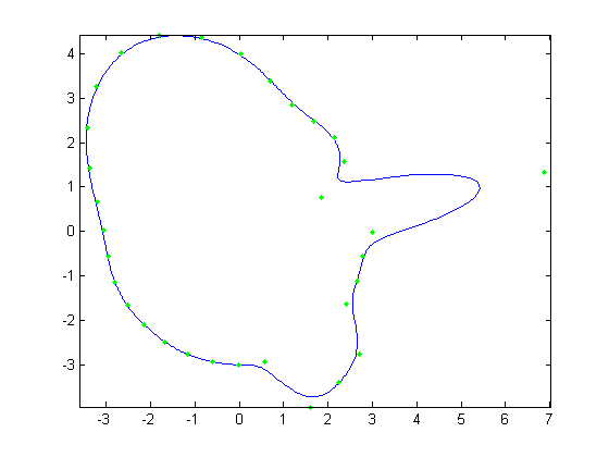
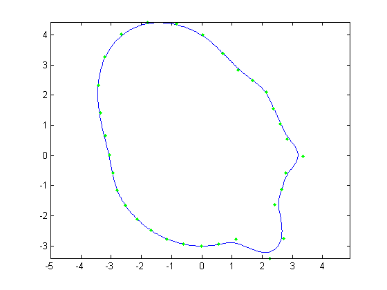
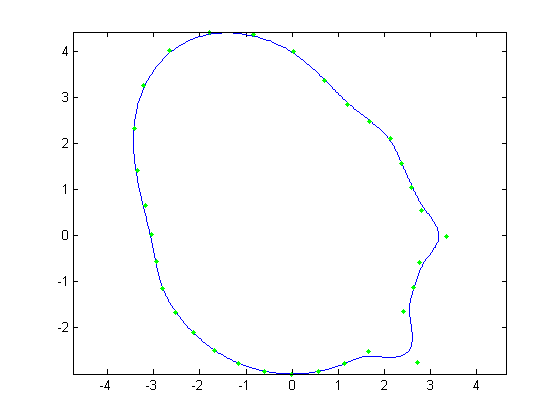
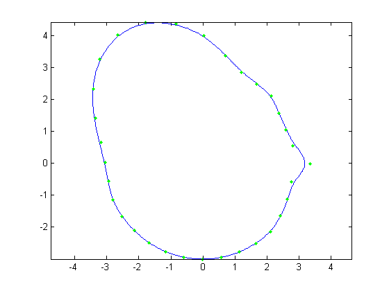
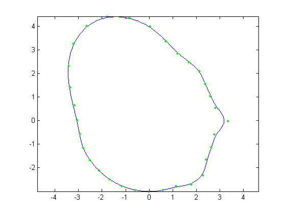
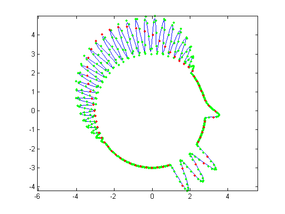
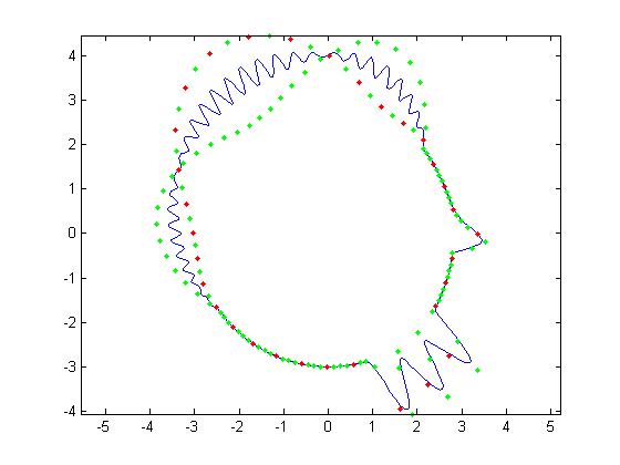
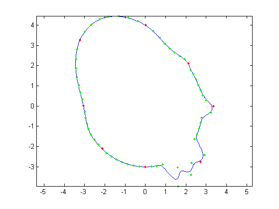
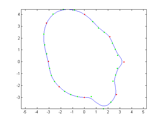
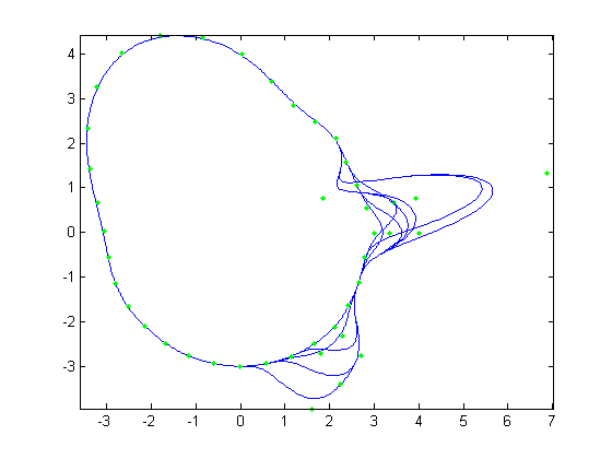
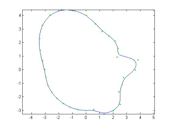
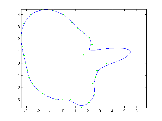
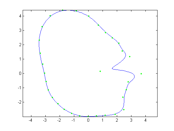
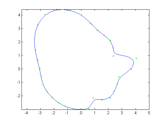
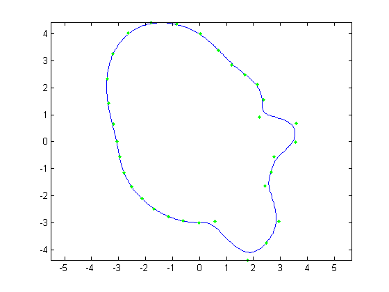
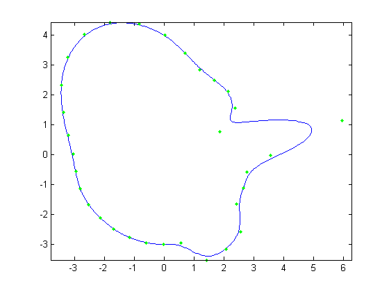
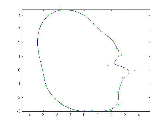
For the first part, the original face was reconstructed with B-Splines using a varying number of control points. Control points varied from
all 512 of the original face, to every other control point, then every fourth, then every eighth and finally every 16th. Below, Figures 1, 3, 5,
7, and 9 show these reconstructions respectively. The blue line is the reconstructed curve, the green dots are the control points used, and the red
dots relate to the FFT and will be discussed shortly. As we decrease the number of samples, we begin to see aliasing problems in the high frequency
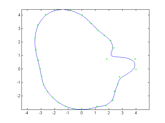
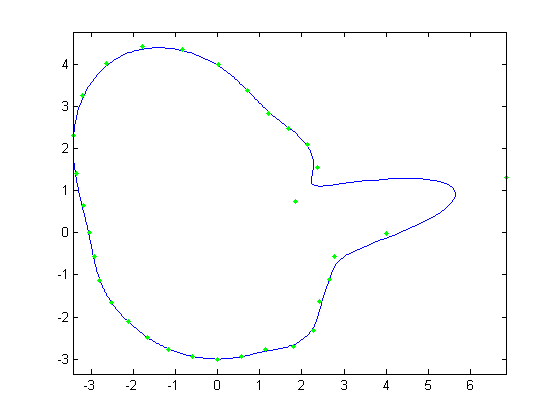
areas of the hair and chin. At 128 samples, the hair looks like two separate low frequency sine waves instead of one high frequency one. At 64 samples,
each sample of the hair hits at approximately the same height on each iteration of the sine wave creating a cone head. The chin still holds some
detail at this point but it is lost at 32 samples. We also notice the nose begins to round off due to less control points being able to describe its
shape.
Part 2
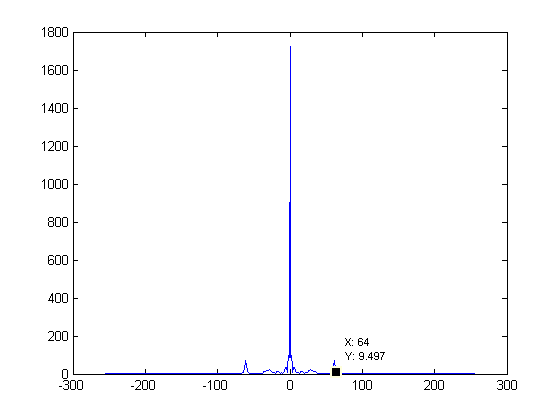
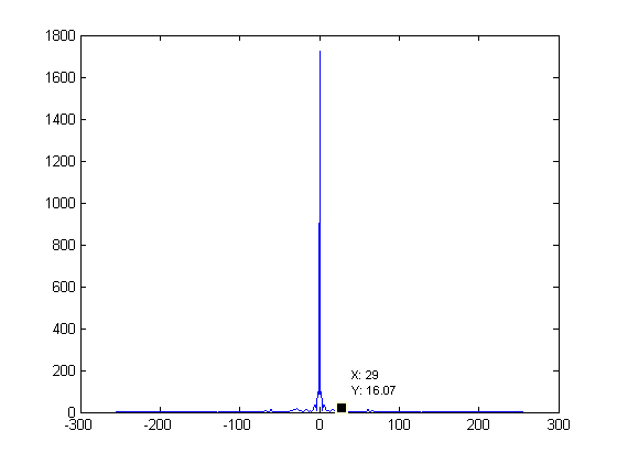
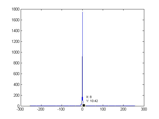
For this part, the FFT of each of the previous set of samples were taken. Figures 2, 4, 6, 8, and 10 show the FFT corresponding to the set of samples to the left.
There are some spikes around 64 on the 512 samples graph. This likely represents the hair since the spikes fall off with less samples.
On each of these graphs the epsilon = 0.01 value is labeled. This value is supposed to help us find the number of samples we need to prevent aliasing.
It is found by locating the highest frequency has 1% of the energy that the zero value has. Since the zero value was around 1700 for all of these graphs, I looked
for values near 17. The red dots mentioned earlier represent the sampling recommended by this aliasing consideration. These values were rounded up to
the next power of 2, so that it would work out nicely. In my opinion these sample rates do a bad job and would clearly lose all detail in the hair.
As the samples decrease, so does the epsilon value. Interestingly, it only has 3 steps. A value of 64 seems to represent that it is trying to preserve
the hair. A value of 32 seems to deal with the beard as it is almost gone. A value of 8 represents the face itself, as once the beard detail is lost,
epsilon sits at 8.
 |
 |
| Figure 1. 512 control points |
Figure 2. FFT of Fig. 1 |
 |
 |
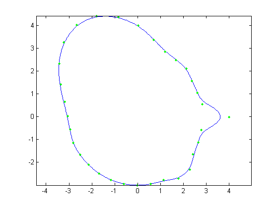
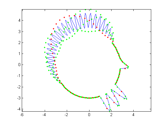
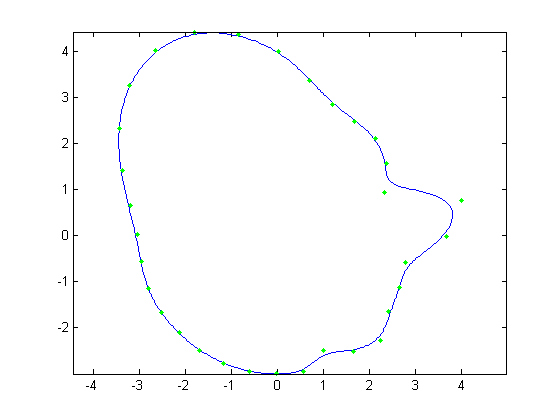
| Figure 3. 256 control points |
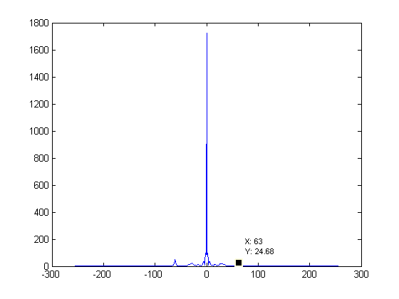
Figure 4. FFT of Fig. 3 |
 |
 |
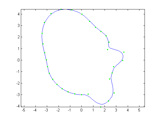
| Figure 5. 128 control points |
Figure 6. FFT of Fig. 5 |
 |
 |
| Figure 7. 64 control points |
Figure 8. FFT of Fig. 7 |
 |
 |
| Figure 9. 32 control points |
Figure 10. FFT of Fig. 9 |
Part 3
In part 3, I created 12 new faces from the 32 samples face. These can be seen below. There are 5 faces that have nose alterations, 4 that have
chin alterations, and 3 that have both. I have also shown a depiction of all the faces drawn on top of each other for reference. After these
twelve faces were created, the average face was calculated and can be seen in Figure 11. Then, Principal Component analysis was done to determine
the main attributes of the faces. Figures 12 through 15 show the mean face +/- 2 std deviations in the first and second principal directions. Figures
16 through 19 show the mean face +/- sqrt(2) std deviations in the first and second principal directions. What we see is that the first principal direction
consists primarily of the nose. This is not surprising because there were more nose samples, 2 of which involved a very large Pinocchio nose. Naturally,
the second principal direction seems to be mostly the chin. Something of interest is that both principal directions contain a bit of the nose and chin, even
though the first is predominantly nose and the second is predominantly chin. This is most likely due to the 3 hybrid faces I made that had both nose
and chin modifications.
| All 12 Faces Overlayed |
 |
 |
| Figure 11. The average face |
 |
 |
| Figure 12. Avg face + 2 std dev. in first principal direction |
Figure 13. Avg face - 2 std dev. in first principal direction |
 |
 |
| Figure 14. Avg face + 2 std dev. in second principal direction |
Figure 15. Avg face - 2 std dev. in second principal direction |
 |
 |
| Figure 16. Avg face + sqrt(2) std dev. in first principal direction |
Figure 17. Avg face - sqrt(2) std dev. in first principal direction |
 |
 |
| Figure 18. Avg face + sqrt(2) std dev. in second principal direction |
Figure 19. Avg face - sqrt(2) std dev. in second principal direction |
Grading & Comments
Grading information and comments can be sent to  .
.