1) Bayer Pattern

1. Implementation of the linear interpolation approach: ../my_demosaic.m

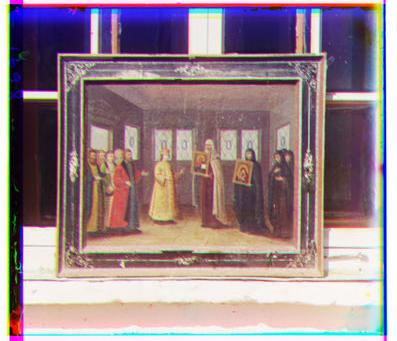
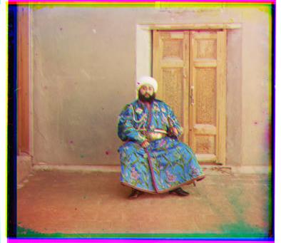
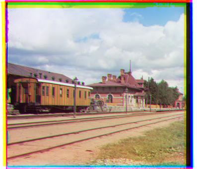
   Figure 1 shows the final result of this approach.

   ---

   
   

   Figure 1: Result of interpolation approach (ignoring the border pixels)

   
   

   Figure 2: Original image

   ---

2. Compute a map of squared differences: shown in Figure 3

   ---

   
   

   Figure 3: Map of Squared Differences

   ---

3. Compute average and maximum per-pixel errors (squared difference) for the image:
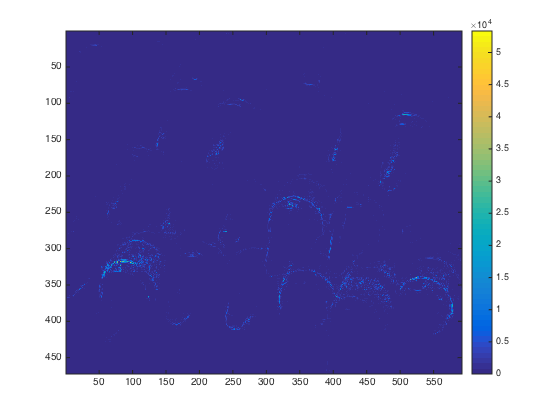
   average summed squared difference per pixel error: 146.452544
   max summed squared difference per pixel error: 53345.125000
4. Show a close-up of a patch of the reconstructed image where the artifacts are particularly apparent and explain the cause of these artifact: An close-up patch shown in Figure 4. There are some zipper artifacts and color inconsistency artifacts. The zipper artifacts are caused because that unknown values at Green pixels in a way that is inconsistent with how it computes unknown values at ted and blue pixels. The color inconsistency artifact is caused because the color change over a small area so that the algorithm cannot get the exact value of the color.

   ---

   
   

   Figure 4: close-up

   ---

2) Image Alignment

1. ncc_align.m is the implementation of single-scale alignment using NCC
   multiscale_align.m is the implementation of multi-scale alignment using SSD (call the function ssd_align.m to compute single-scale alignment using SSD)
2. The result images and the (y, x) displacement vector that was used to align the channels are shown in the following.

   ---

   
   

   Figure 5: 00125v.jpg: Displacement Vector(y, x): Red (3, -2), Blue (-6, -3)

   ---

   ---

   
   

   Figure 6: 00149v.jpg: Displacement Vector(y, x): Red (4, -1), Blue (-5, -3)

   ---

   ---

   
   

   Figure 7: 00153v.jpg: Displacement Vector(y, x): Red (6, 1), Blue (-8, -4)

   ---

   ---

   
   

   Figure 8: 00351v.jpg: Displacement Vector(y, x): Red (8, 0), Blue (-5, -2)

   ---

   ---

   
   

   Figure 9: 00398v.jpg: Displacement Vector(y, x): Red (5, 0), Blue (-6, -4)

   ---

   ---

   
   

   Figure 10: 01112v.jpg: Displacement Vector(y, x): Red (4, 0), Blue (-1, -1)

   ---

   ---

   
   

   Figure 11: 01047u.tif: Displacement Vector(y, x): Red (46, 13), Blue (-25, -21)

   ---

   ---

   
   

   Figure 12: 01657u.tif: Displacement Vector(y, x): Red (61, 3), Blue (-55, -10)

   ---

   ---

   
   

   Figure 13: 01861a.tif: Displacement Vector(y, x): Red (75, 23), Blue (-72, -39)

   ---

3. Multi-scale alignment.

   ---

   

   

   

   
   

   Figure 14: Single-scale Alignment Using NCC

   ---

   ---

   

   

   

   
   

   Figure 15: Multi-scale Alignment Using SSD

   ---

   The displacement vectors of all the high-resolution pictures using multi-scale alignment method with SSD are displayed as follows.

   1. 01047u.tif: Displacement Vector(y, x): Red (47, 14), Blue (-24, -19)
   2. 01657u.tif: Displacement Vector(y, x): Red (61, 3), Blue (-49, -8)
   3. 01861a.tif: Displacement Vector(y, x): Red (76, 24), Blue (-71, -38)

   ---

   Method	01047u.tif	01657u.tif	01861a.tif
   Single-scale Alignment Using NCC	40.624939	38.174243	39.717424
   Multi-scale Alignment Using SSD	3.388226	4.741146	3.333986

   
   

   Table 1: Comparison of Time (Seconds)

   ---