Figure 1: Least Squares for Line1
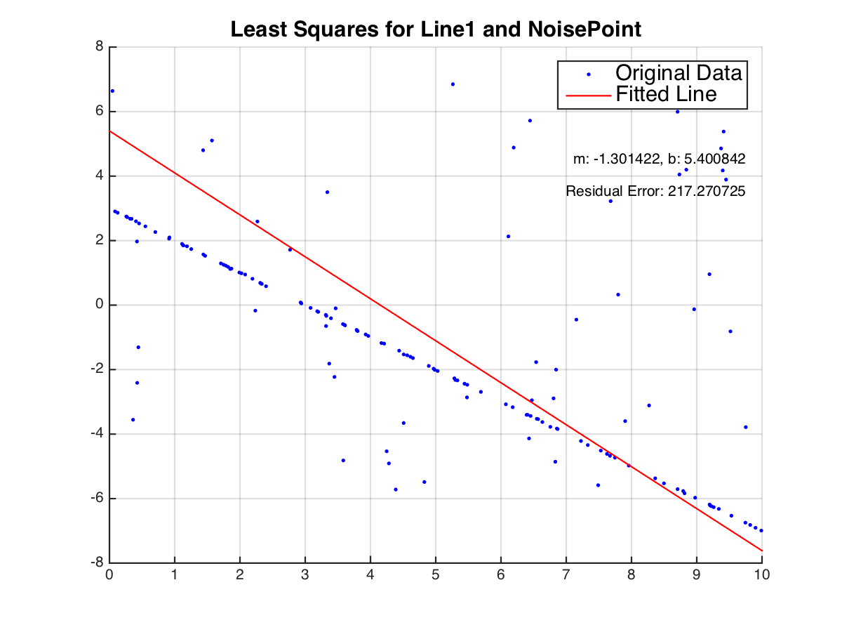
Figure 2: Least Squares Line1 and
NoisePoint
Notice
The perpendicular distances are used while calculating the residual error and Least Square method. Code for the assignment is assign3.m
Least Squares
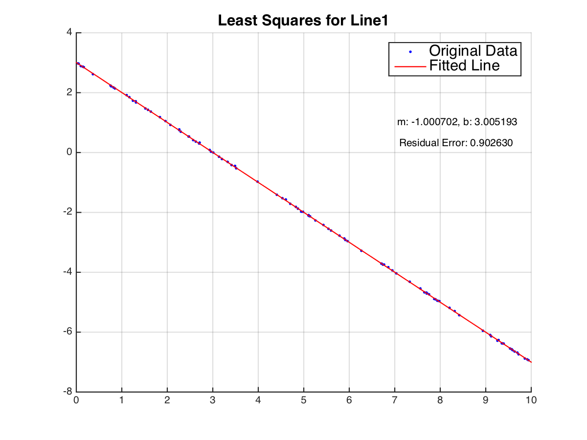
1) Estimate the line parameters m,b of the line l1 for the mx + b = y from the dataset returned by function Line1 using least squares. Plot the points and the fitted line and report the residual error for the fit, i.e. the sum of the squared distances of the points to the line.
2) Then repeat the above fit one hundred times and provide the mean and variance for the estimated parameters.
3) Estimate the line parameters m,b of the line l1 for the mx + b = y using least squares from the
dataset joining the outputs of the function Line1 and NoisePoints. Plot the points and the fitted line
and report the residual error for the fit, i.e. the sum of the squared distances of the points to the
line.
Solution: least_square.m
1) Figure 1 shows the original points generated from Line1 and the fitted line using Least Squares Method. The residual error is also shown in the figure.
2) The results of training one hundred times:
The mean of m is -0.999953, and variance of m is 2.35e-07
The mean of b is 2.999572, and variance of b is 7.54e-06
3) Figure 2 illustrates the points with noise, the fitted line using Least Squares Method and the residual error of the fitting.
RANSAC
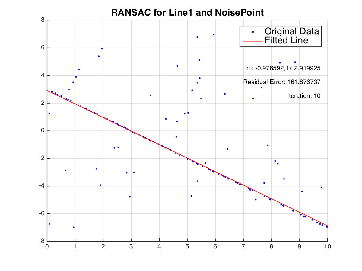
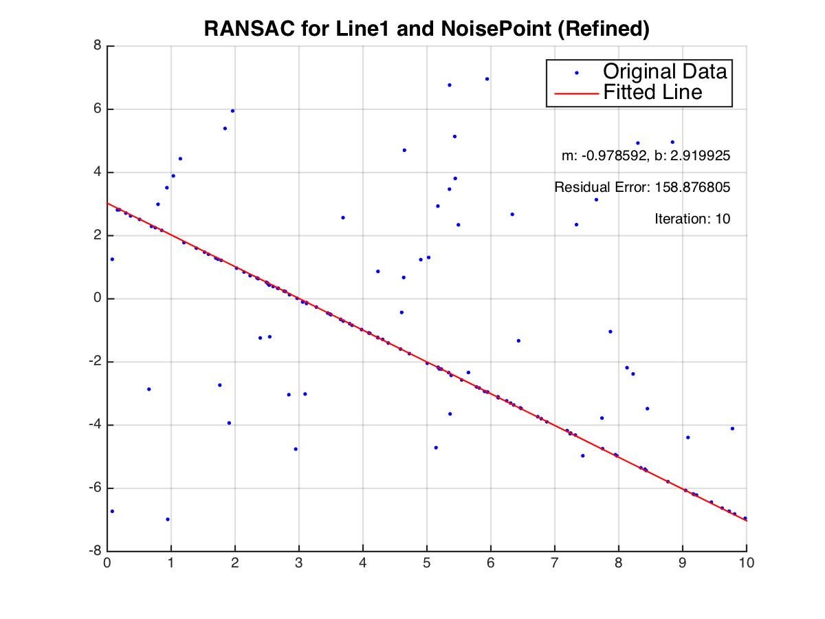
1) Estimate the line parameters m,b of the line l1 for the mx + b = y using RANSAC (using adaptive stopping) from the dataset joining the outputs of the function Line1 and NoisePoints. Also use the above least squares fit to refine the RANSAC solution by computing the final solution as least squares fit over the inliers. Report the number of RANSAC iterations needed to compute the solution. Plot the points and the fitted line and report the residual error for the fit, i.e. the sum of the squared distances of the points to the line.
2) Then repeat the above RANSAC fit one hundred times and provide the mean and variance for
the estimated line parameters and the number of required RANSAC trials.
Solution: ransac.m
1) Figure 3 shows the outputs including errors and iterations of the points fitted by RANSAC. Figure 4 demonstrated the results refined by Least Squares method.
2) The results of training one hundred times:
The mean of m is -1.007451, and variance of m is 8.90e-04
The mean of b is 3.044426, and variance of b is 3.12e-02
The mean of # RANSAC trials is 8.260000, and variance of # RANSAC trials is
3.12e+00
Hough Transformation
1) Estimate the line l2 for the dataset returned by function Line2 using the Hough Transform. Plot the points and the fitted line.
2) Simultaneously, estimate the lines l1,l2 for the dataset returned by function Line1 and Line2 using the Hough Transform, respectively. Plot the points and the fitted lines. What is the difference of the line fits?
Solution: hough_transformation.m
1) Figure 5 illustrates the points generated by Line2 and the fitted line using Hough Transformation method.
2) Figure 6 shows points returned from Line1 and Line2 and the fitted lines. There is no difference between the fitted line in part 1) and one of the fitted lines in this part.
Summary:
Table 1 and 2 demonstrate the comparison of the fitting using three different methods, namely
Least Squares, RANSAC, Hough Transformation, for Line1 and Line1 with NoisePoints
respectively. We repeat the whole process of line fitting for 100 times. μ is the mean and
σ2 is the variation of the parameter. The time is the total computation time for the 100
experiments.
| Methods | μm | σm2 | μb | σb2 | time(s) |
| Least Squares | -0.999953 | 2.35 × 10⁻⁷ | 2.999572 | 7.54 × 10⁻⁶ | 0.049947 |
| RANSAC | -0.996163 | 6.69 × 10⁻⁴ | 2.983278 | 2.11 × 10⁻² | 0.010076 |
| Hough Transformation | -1.000000 | 0.00 | 2.969848 | 1.99 × 10⁻³¹ | 0.488400 |
| Methods | μm | σm2 | μb | σb2 | time(s) |
| Least Squares | -1.357599 | 1.42 × 10⁻² | 5.470084 | 5.80 × 10⁻¹ | 0.059292 |
| RANSAC | -1.007451 | 8.90 × 10⁻⁴ | 3.044426 | 3.12 × 10⁻² | 0.040483 |
| Hough Transformation | -1.000000 | 0.00 | 2.969848 | 1.99 × 10⁻³¹ | 0.448514 |
Analysis: