Validation using Synthetic Applications

The data analysis techniques described in the previous section are based on a number of properties of TCP that are expected to hold for the vast majority of connections recorded. For example, the logical data order property should always hold, since TCP would fail to deliver data to applications otherwise. There are, however, a number of possible sources of uncertainty in the accuracy of the data acquisition method, and this section studies them using testbed experiments.

The concept of an ADU provides a useful abstraction for describing the demands of applications for sending and receiving data using a TCP connection. However, the ADU concept is not really part of the interface between applications and TCP. In practice, each TCP connection results from the use of a programming abstraction, called a socket, that receives requests from the applications to send and receive data. These requests are made using a pair of socket system calls, send() (application's write) and recv() (application's read). These calls pass a pointer to a memory buffer where the operating system can read the data to be sent or write the data received. The size of the buffer is not fixed, so applications are free to decide how much data to send or receive with each call and can even use different sizes for different calls. As a result, applications may use more than one send system call per ADU, and there may be significant delays between successive calls belonging to the same ADU. These operations can further interact with mechanisms in the lower layers (e.g., delayed acknowledgment, TCP windowing, IP buffering, etc.) creating even longer delays between segments carrying ADUs. Such delays distort the relationship between application-layer quiet times and segment dynamics, complicating the detection of ADU boundaries due to quiet times.

To test the accuracy of our data acquisition techniques, we constructed a suite of test applications that exercise TCP in a systematic manner. The basic logic of each test application is to establish a TCP connection and send a sequence of ADUs with a random size, and with random delays between each pair of ADUs. In the a-b-t model notation, this means creating connections with random $a_i$ , $b_i$ , $ta_i$ and $tb_i$ . As the test application runs, it logs ADU sizes and various time intervals as measured by the application. In addition, the test application can set the socket send and receive calls to random I/O sizes, and can introduce random delays between successive send or receive calls within a single ADU. In our experiments, the test application was run between two real hosts, and traces of the segment headers were collected and analyzed using our measurement tool. Our validation compared the result of this analysis and the correct values logged by the applications.

**Figure 3.12:** Distributions of ADU sizes for the testbed experiments with synthetic applications.
$\includegraphics[width=3in]{fig/tcp2cvec-limitations/limitations-adu.body.eps}$

**Figure 3.13:** Distributions of quiet time durations for the testbed experiments with synthetic applications.
$\includegraphics[width=3in]{fig/tcp2cvec-limitations/limitations-t.body.eps}$

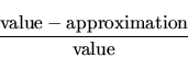
We conducted an extensive suite of tests, but limit our report to only some of the results. Specifically we only show the results with the most significant deviations from the correct values for ADU sizes or quiet time durations. Figure 3.12 shows the relative error, defined as

$\begin{displaymath}\frac{\mathrm{value} - \mathrm{approximation}}{\mathrm{value}} \end{displaymath}$

In general, we found only two cases that expose limitations in the data acquisition method when analyzing sequential connections. While random application-level send and receive sizes, and random delays between successive send operations within a data unit do not have a significant effect, random delays between successive receive operations produce errors in estimating some quiet time durations. In this case, the application inflates the duration of a quiet time by not reading data that may already be buffered at the receiving endpoint. The consequence is a difference between the quiet time as observed at the application level and the quiet time observed at the segment level. The quiet time observed by the application is the time between the last read used to receive the ADU $a_i$ (or $b_i$ ) and the first write used to send the next ADU $b_i$ ( $a_{i+1}$ ). The quiet time observed at the segment level is the time between the arrival of the last segment of $a_i$ ( $b_i$ ) and the departure of the first segment of $b_i$ ( $a_{i+1}$ ). If the application reads the first ADU slowly, using read calls with significant delays between them, it will finish reading $a_i$ ( $b_i$ ) well after the last segment has reached the endpoint. In this case, the quiet time appears significantly shorter at the application level than at the segment level.

For example, a data unit of 1,000 bytes may reach the receiving endpoint in a single segment and be stored in the corresponding TCP window buffer. The receiving application at this endpoint could read the ADU using 10 recv() system calls with a size of only 100 bytes, and with delays between them of 100 milliseconds. The reading of this ADU would therefore take 900 milliseconds, and hence the application would start measuring the subsequent quiet time 900 milliseconds after the arrival of the data segment. Our measurement of quiet time from segment arrivals can never see this delay in application reads, and would therefore add 900 milliseconds to the quiet time. For most applications we claim there is no good reason to delay read operation more than a few milliseconds. Therefore, the inaccuracy demonstrated here should be very infrequent. Nonetheless we have no direct means of assessing this type of error in our traces.

Figure 3.13 shows the relative error in the measurement of quiet time duration when there are random delays between successive read operations. The worst error is found when measuring quiet times between $a_i$ and $b_i$ (i.e., within an epoch) when random read delays occur on the connection acceptor (receiver of $a_i$ and $b_i$ ). Even in this case, 70% of values have less than 20% error in an experiment with what we considered severe conditions of delays between read operations for a single ADU (random delays between 10 and 100 milliseconds).

We also studied the impact of segment losses on the accuracy of the measurements. In general, the algorithm performs well, but the analysis helped us to identify one troublesome case. If the last segment of an ADU is lost, the receiver side does not acknowledge the last sequence number of the ADU. After a few hundred milliseconds the sender side times out and resends the last segment. If the loss of the segment occurs before the monitoring point, no retransmission is observed for this last segment. If the time between this last segment and its predecessor is long enough (due to the TCP timeout), the ADU is incorrectly divided into two ADUs. Other types of segment loss do not have an effect on the measurement, since the algorithm can use the observation of retransmission and/or reordering to identify quiet times not caused by source-level behavior. The troublesome case is so infrequent that we did not try to address it. However, we note that it seems possible to develop a heuristic to detect this type of problem. The idea would be to estimate the duration of the TCP retransmission timeout, and ignore gaps between segments that are close to this estimate. The implementation of this heuristic would be complicated by the need to take into account differences in the resolution of the TCP retransmission timers, round-trip time variability and the possibility of consecutive losses.

**Figure 3.14:** Distributions of ADU sizes for the testbed experiments with synthetic applications.
$\includegraphics[width=3in]{fig/tcp2cvec-limitations/limitations-conc-adu.body.eps}$

**Figure 3.15:** Distributions of quiet time durations for the testbed experiments with synthetic applications.
$\includegraphics[width=3in]{fig/tcp2cvec-limitations/limitations-conc-t.body.eps}$

Measuring the size of ADUs in concurrent connections is generally more difficult. This is because a change in the directionality of sequence number increases does not constitute an ADU boundary and thus we have to rely instead on quiet times to split data into ADUs. Figure 3.14 compares the input distribution of ADU sizes (from both a-type and b-type ADUs) and the measured sizes when the sizes of socket reads/writes and the delays between them are random. The measurement is generally very accurate, although some ADUs that were sent with small quiet times between them are mistakenly joined into the same measured ADU. This creates a longer tail in the measured distributions. Reducing the quiet time threshold from 500 to 250 milliseconds does little to reduce the measurement inaccuracy.

The measured quiet times are also quite close to those at the application level, as shown in Figure 3.15. The small inaccuracy comes again from ADUs that are joined together when their inter-ADU times are short. This inaccuracy biases the measured distribution of quiet times against small values (notice that the measured distributions start at a higher value). Reducing the minimum quiet time threshold to 250 milliseconds makes the measured distribution closer to the actual distribution.