COMP 790 - Project: Photofractals

COMP 790 - Project: Photofractals

Ryan Schubert
Fall, 2008

Project proposal and previous progress updates can be found here.

Core Idea
The core idea for this project is the following: given two input photos, image1 and image2, find a patch of image1 that best matches a scaled-down version of image2. In the case where the same image is used for both image1 and image2, this results in finding a small, self-similar patch of the image--this was the original idea and the motivation behind the name "photofractals". Because there aren't necessarily going to be good matches between any arbitrary pair of input images, if we want to find particularly good matches we either need a user to manually select probable looking candidates or we can provide a large collection of input images and automatically find the good matches between pairs of images in the input set. One of the motivations for this project was being able to automatically find similarities that were non-obvious to a human, so an automatic approach was preferable.

Overview
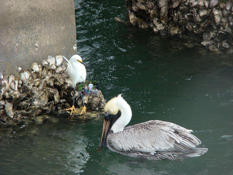
The expected sort of dataset that would be used as the input for this system would be a collection of related digital photos, such as those taken on a trip or visit to a certain place. The dataset that was used for testing this system was the first 128 images of 200 total images that I took while in Florida visiting relatives. The cutoff at 128 images was arbitrary and simply for the sake of limiting the runtime and memory usage. The full dataset is available here.

For larger input datasets we cannot compute the best sub-patch match for all possible ordered pairs of input images. This would take far too long, so we must instead find a much faster way of finding the top potential matches within the total set of images, and then we can find actual matches within that subset. The first pass of the system computes the color histograms for all images and then populates a lower diagonal matrix with the sum of squared distances between histograms for all pairs of input images. We can then consider only the top N lowest SSD image pairs for computing the actual best sub-patch match. This relies on the assumption that images for which the color histograms are significantly different will probably not match well anywhere inside each other.

Once we have reduced the number of comparisons down to the top N lowest SSD image pairs, we can actually compute the best sub-patch matches for all N pairs, in both directions (since order does matter now, while it did not for the histogram SSD). Originally this step involved computing the per-pixel L2 distance in RGB and gradient space for all possible sub-patch locations within the target image. This took on the order of 2 minutes for a single patch scale for an 816x612 image--too slow to do all 2N comparisons for reasonable values of N. We can get a decent approximation by using normalized cross-correlation instead. Normalized cross-correlation is defined as:

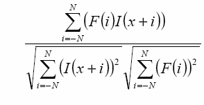
Where -N to N is the pixel neighborhood of the template patch and I(x) is the current patch location in the target image.

It is also nicely invariant to scaling the intensity of either the template or the image. Computing the normalized cross-correlation for all possible patch locations took on the order of 6 seconds, compared to the 2 minutes for computing actual L2 distance.

Also at this step the background image was blurred before computing the gradient. The intension here was an attempt to preserve the larger structure in an image rather than trying to match local noisy texture information (e.g. we'd rather match the edge between grass and a road rather than trying to match the gradient of the grass or asphalt texture as much).

Originally the actual max normalized cross-correlation responses were used as a measure of "how good" the resulting ordered pair match was. Looking at the top 20 matches we can see that this results in some good matches and some that seem pretty poor.

At this point an additional step was added in an attempt to better select the best ordered pair matches than just the normalized cross-correlation responses. For this, we computed the pixel-wise SSD (RGB and gradient space) for the sub-patch location determined by the maximum correlation response. Although time-consuming to do for finding the best sub-patch, this is relatively quick to compute for each already determined sub-patch location in all ordered pairs. Using the computed SSDs two different ranking metrics were used: just using the SSD values and using a value that combined the correlation response and the SSD value by computing the ratio of the response to the SSD (where higher responses are better and lower SSDs are better).
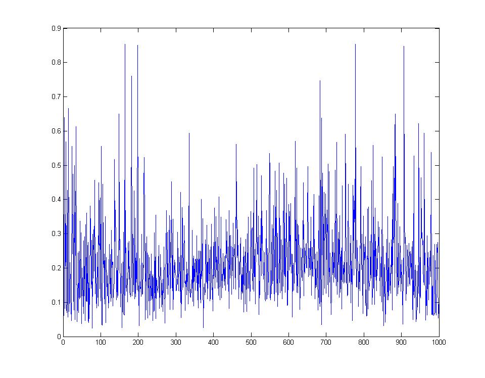
We can see that, in fact, the normalized cross-correlation responses did not seem to correlate with the pixel-wise SSD ranking at all. Here is a graph of the SSDs of 1000 images ordered according to decending normalized cross-corrrelation repsonse:

Using an inverted gaussian to weight the validation SSD results was also tried in an effort to better match the border of the patch with the underlying background, but this did not tend to produce significantly better results, and produced more results where the center of the sub-patch was much more visible in the zoomed out state (regardless of how well it blended).

Generating an Image Sequence
Given a list of ranked, ordered image pairs, we then compute a greedy good path that transitions through some subset of the input images, where each image is embedded in the proceeding image, allowing for a slide-show effect where you always zoom into some location of the current image to transition to the next image. Because most of the effort was spent on trying to get better pair-wise matches, the method for generating this image sequence was relatively simple: starting with the best-ranked image pair we simply grow our current sequence by looking for the best ranked image pair that either transitions to the first image of the current sequence or from the last image and does not add a photo that we've already included in the sequence. This is repeated until either the image sequence is long enough or until there are no more valid transitions for which we had calculated the best sub-patch match.

Rendering the Slide-show
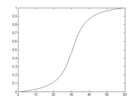
MATLAB was then used to generate proof-of-concept movies of transitioning through the image sequence. Originally very simple linear alpha blending was used (based on the shortest x or y pixel distance from the edge of the patch), which was a marked improvement over no blending at all. Later, a re-sized, clamped gaussian was used as an alpha mask to radially blend patches into the background images. The MATLAB script also allows for generating frames based on a parameter that varies from 0 to 1, where 0 is the background image at full resolution and size and 1 is fully zoomed into the sub-patch. This allowed for smoother zoom transition by varying the parameter according to a re-scaled segment of the arctangent function:

Results
Final slideshow movie - Note this is 189 MB in size, and 11 minutes long. It contains 55 photo transitions (so 56 images total), and was the sequence generated from looking at the top 3000 lowest color histogram image pairs and calculating the corresponding 6000 best sub-patch matches via normalized cross-correlation, and finally ranked by the response/SSD. The sequence and movie were generated using the MATLAB scripts at the bottom of this document. Two arbitrary transitions (that are towards the end of the full final movie) that I thought worked well are:
show_55_parial_45.avi - 4.2 MB
show_55_parial_46.avi - 4.5 MB

Possible Improvements or Future Work
There are a number of possible improvements to this system, depending on the desired goals. When computing the color histogram SSDs as a first-pass on the data, it might actually make more sense to take order into account for each pair since as long as one image's color histogram is a subset of the other, there is still a chance there could exist a good match. For example, a picture of a person surrounded by green grass might actually have a good matching location within part of another picture of a parking lot that has a grassy field next to it, even though the parking lot picture's color histogram might be significantly different in the red and blue channels. Another first-pass method that would greatly increase the flexibility of sequence generation would be to do actual normalized cross-correlation on significantly low res versions of both the background images and the templates (i.e. such that the templates are 4x4 images). While this would likely not provide any useful prediction for gradient-space matching, it would give a first-pass color comparison and would even allow for a full correlation matrix to be computed for all images in the input dataset, which could then be used for more sophisticated methods of generating lowest energy sequences through as many images as possible. This method could even be applied iteratively with larger templates each time, looking at only the top N best responses at each iteration. Significant improvements could also be made in the slide-show rendering. The MATLAB movie generation was really intended only as a proof-of-concept solution, and there are very noticeable artifacts, namely in the fact that the background and subpatch positions are not resampled to give smooth movement. This became especially apparent after adding the arctan transition function, as this caused frames in which there was little change in the zoom, but often result in full-pixel jumps in the images. An application with real hardware graphics support, such as an OpenGL application, would result in much smoother animation and blending, and could generate frames of video much more quickly than the custom-written MATLAB routines.

MATLAB code:
testdist.m - script that does the following:
- loads the dataset images
- computes the image histogram similarity matrix (this calls imgdist() found in imgdist.m)
- computes the ranked list of the best N potential image pairs
- computes the actual normalized cross-correlation responses between the top N*2 ordered pairs (this calls calcpatch() found in calcpatch.m)
- computes the SSD of the resulting sub-patch match (this calls verify() found in verify.m)
- saves the list of final ordered pairs ranked by the response/SSD values

zoom2.m - zoom2( im1, im2, subx, suby, scale, t, blendw ) generates the image resulting by embedding im2 at the specified scale in im1 at location subx, suby, parameterized by t and with a blendwidth of blendw (where blendw = 1 is 'fully' blended using the gaussian alpha mask and blendw = 0 is such that only the sub-patch pixels are visible and intermediate values work as expected). This function calls embed().
embed.m - embed( dest, patch, subx, suby, blendwidth ) blends the specified patch into dest at location subx, suby with blendwidth as described above.

buildchain.m - simple script that assumes the existence of the ssds matrix generated at the end of testdist.m and builds an image sequence from the ranked list of ordered pairs as described in the Generating an Image Sequence section above.

cmm.m - script that renders and combines movies of each zooming transition in the image sequence generated by buildchain.m. This calls the mm.m script.
mm.m - script that renders a 3-part movie for a single given ordered image pair. Part 1 zooms from image1 to embedded image2 according to the arctan transition function. Part 2 linearly fades out the blending width until only the sub-patch is left. Part 3 adds additional frames identical to the last frame from part 2, such that the photo is visible in its entirety for some duration of time before the next zoom-in occurs.

bestmatches.m - simple script to display the top 20 ranked image pairs
showmatch.m - showmatch( i, matches, images ) is a simple function that calls zoom2 to display the embedded match corresponding to index i, from the list of matches given by matches which indexes into images for the actual image data.