1.1 Description:

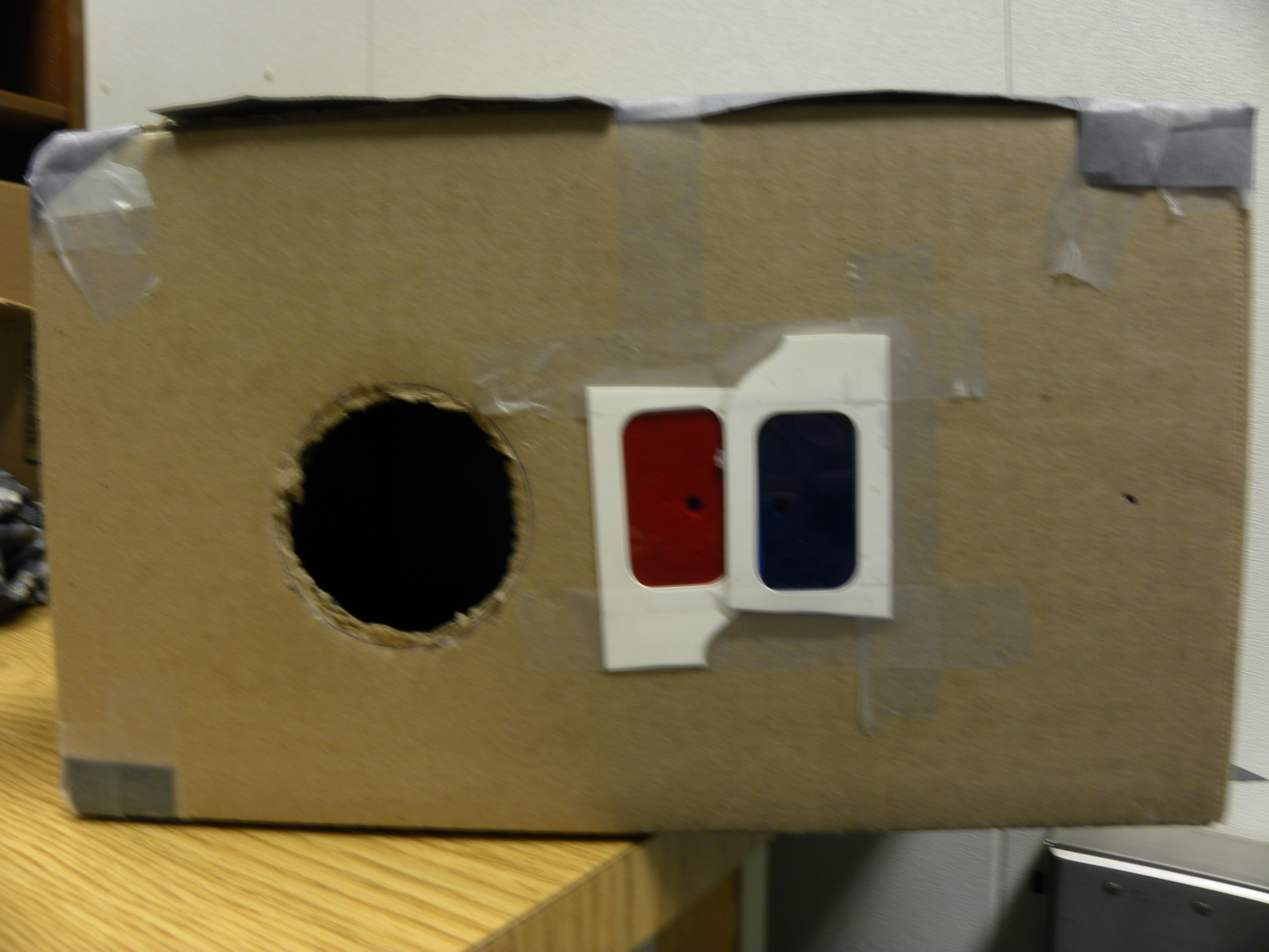
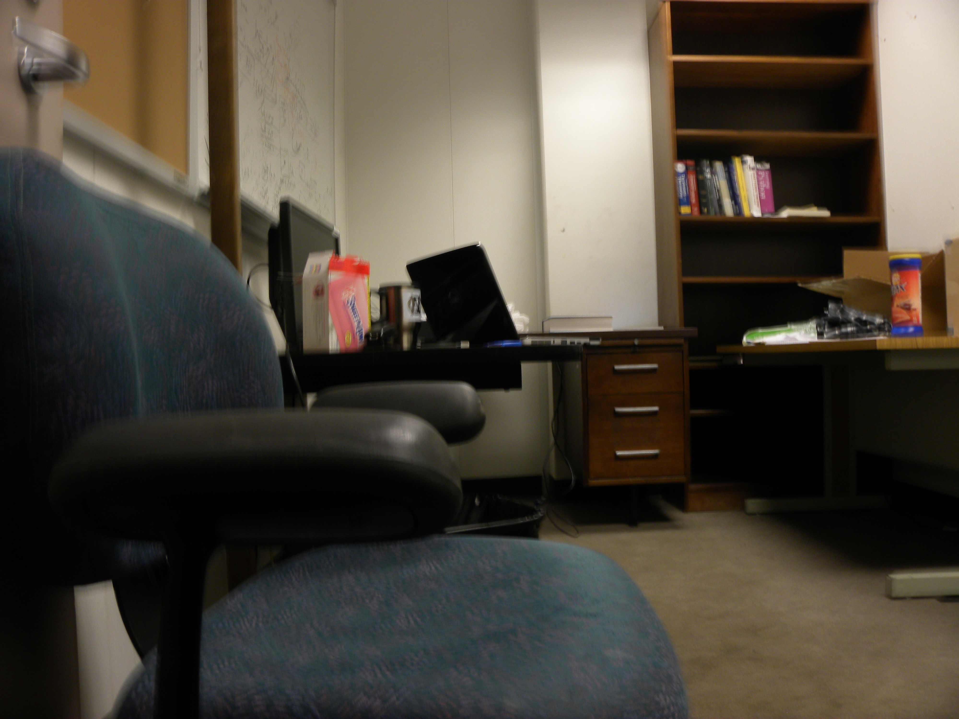
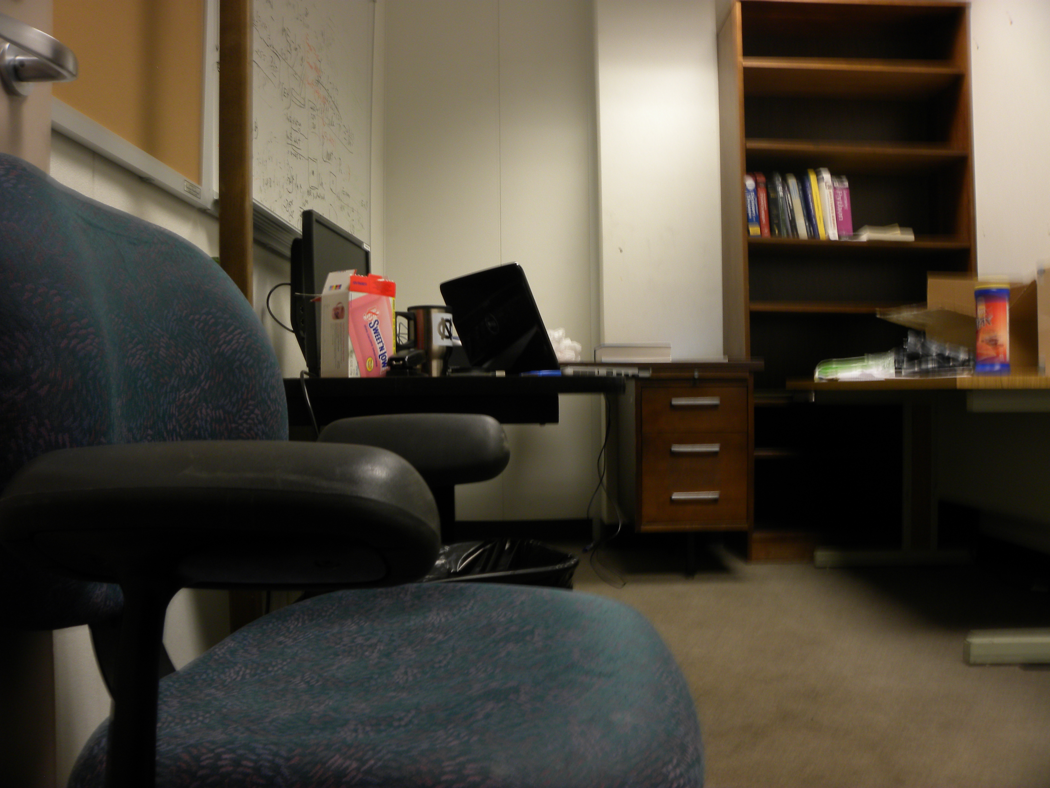
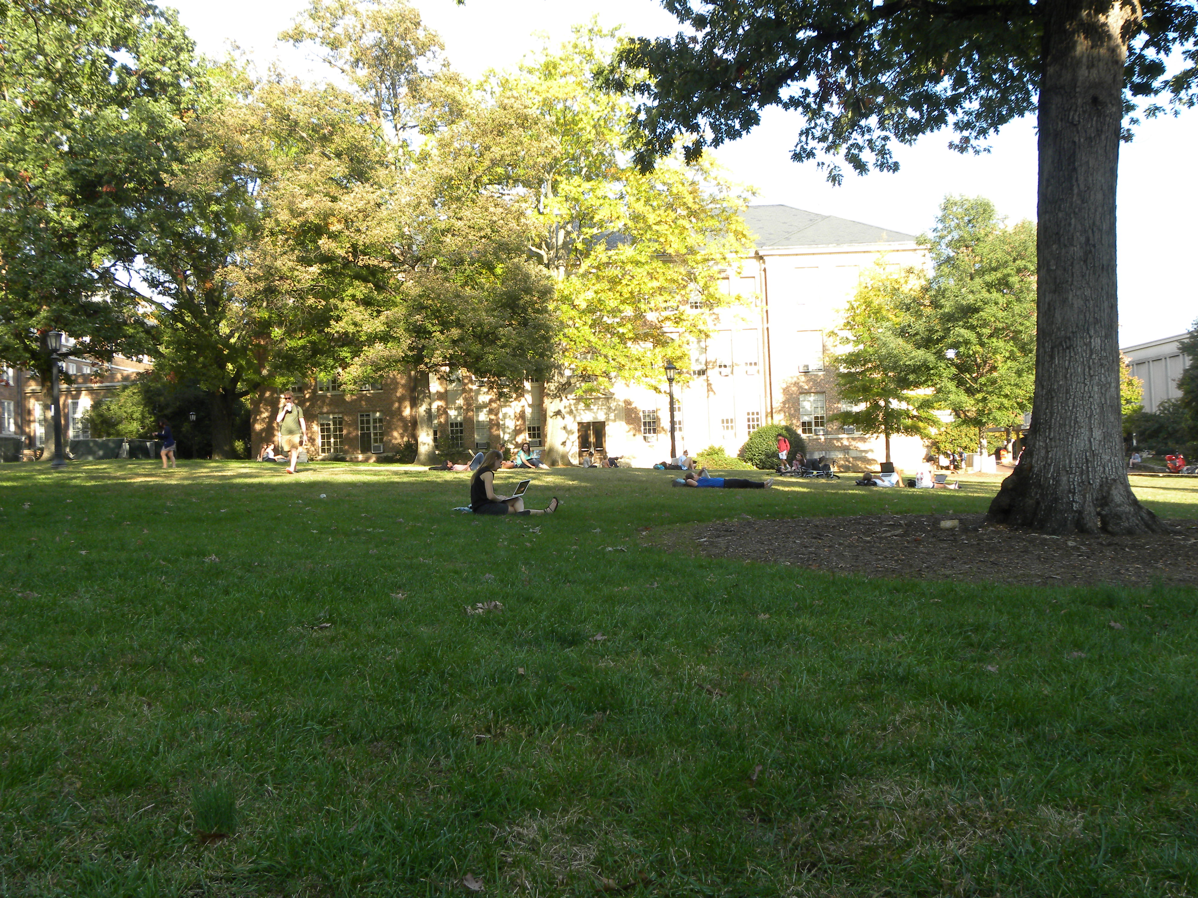
The objective was to construct a stereo pinhole camera using the material provided (filters, black paper,etc Thanks Prof. Berg!) and a shoebox. With the help of the pinhole anaglyph images, 3D depth estimation was done. The second part consisted of creating antipinhole images and possibly using HDR imaging to improve the SNR.

Credit to my group members: Yi Ren(guy with Nikon P90), Danwei Li,Kecheng Yang.

1.2 Creating the stereo pinhole camera

The shoebox was covered with black paper from inside and one side of the box was glued a white paper which functioned as a screen. All the holes, corners,etc form where light could leak inside were covered with abundant use of tape and black paper.

Fig 1: Stereo pinhole camera

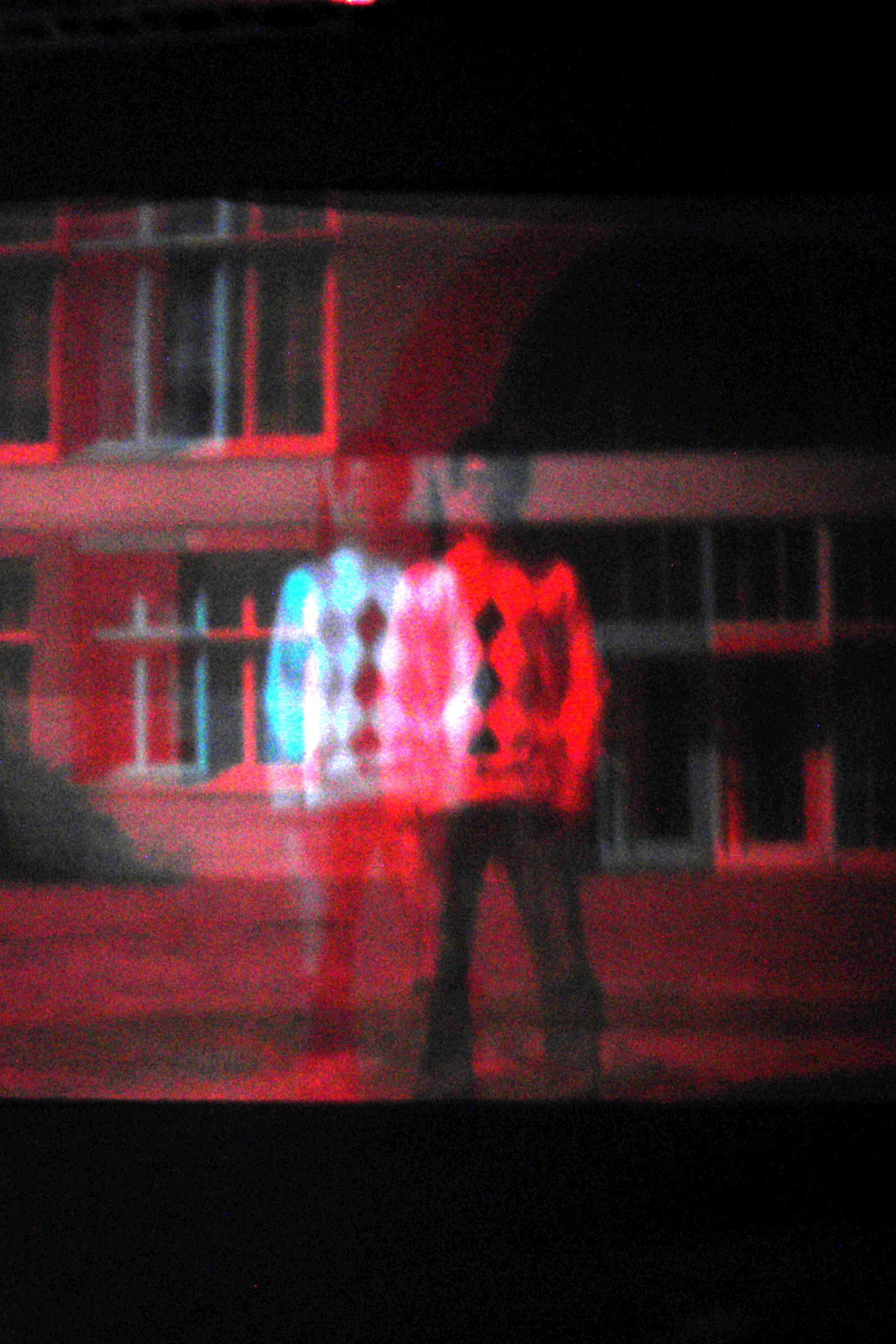
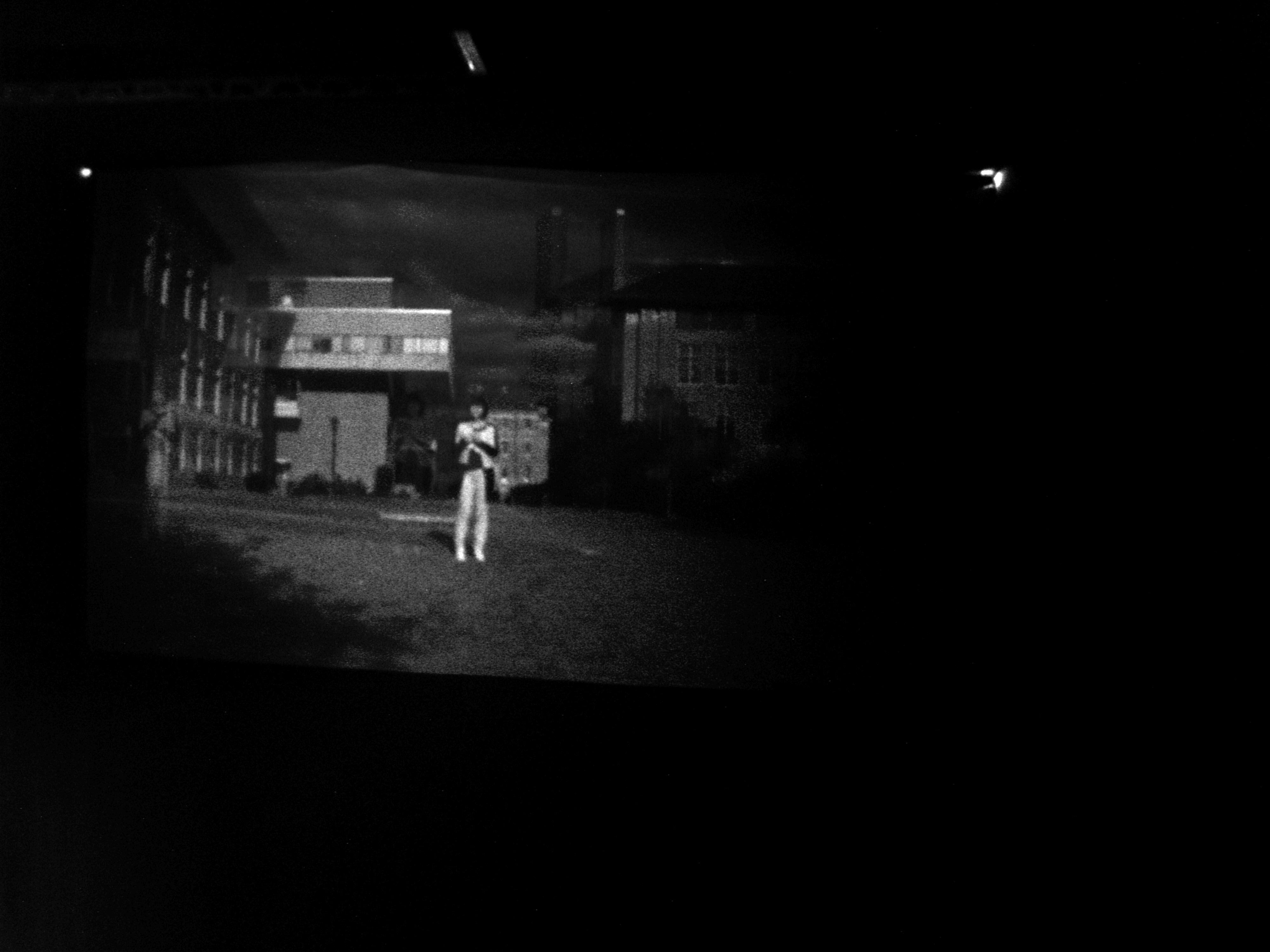
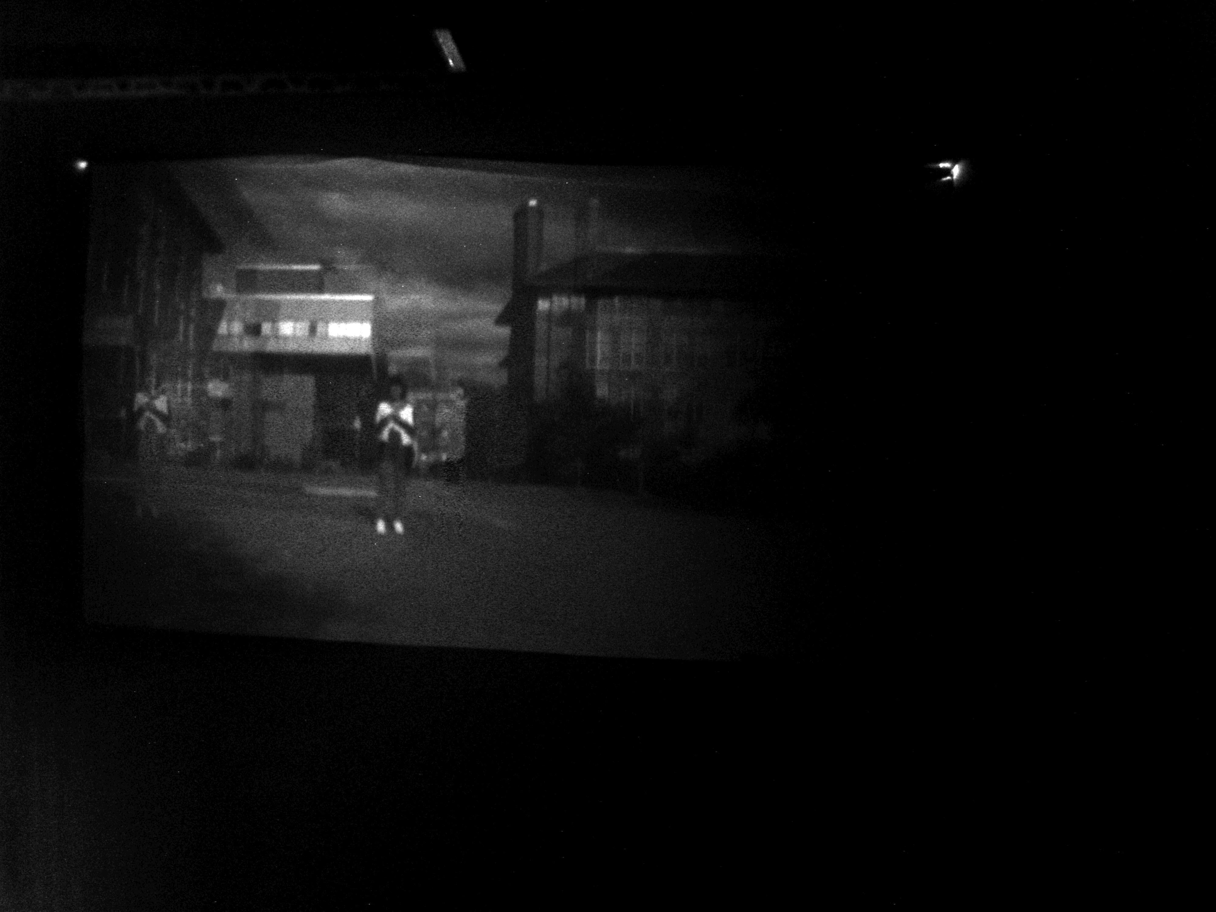
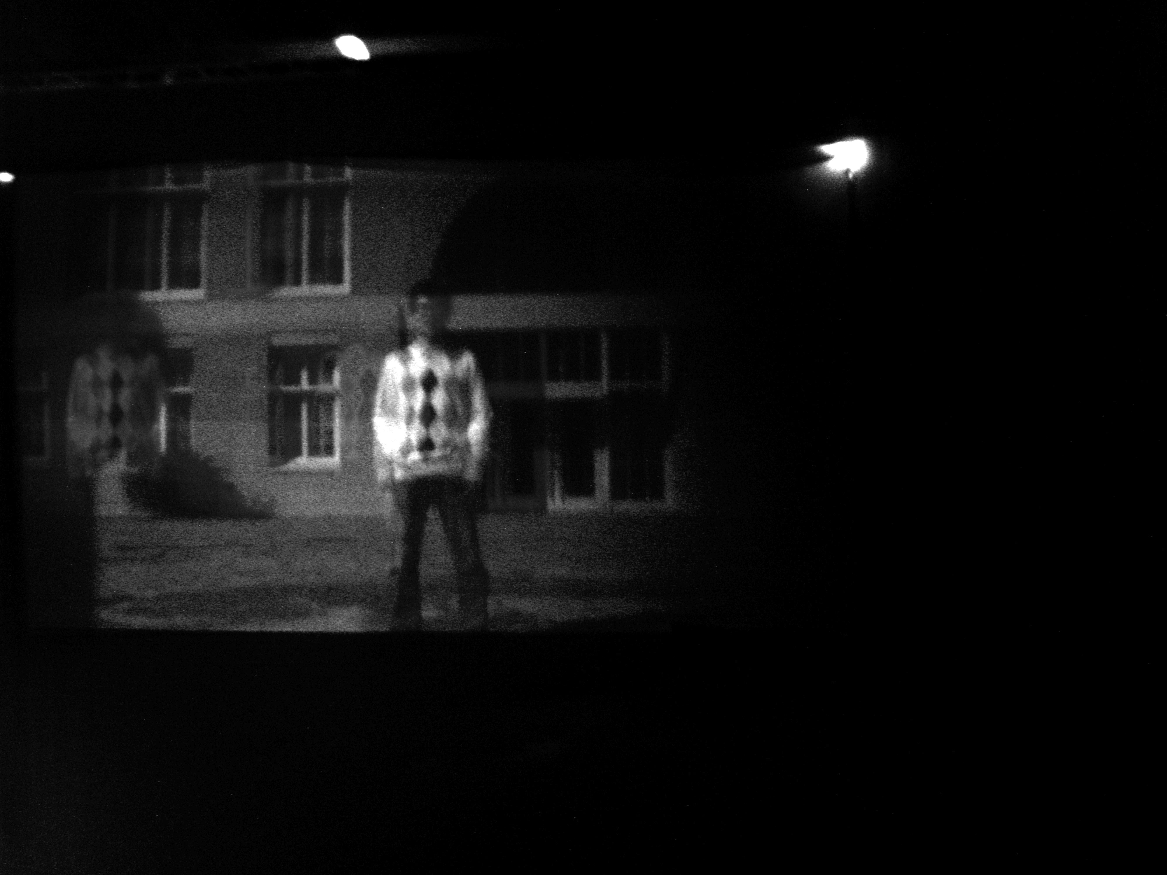
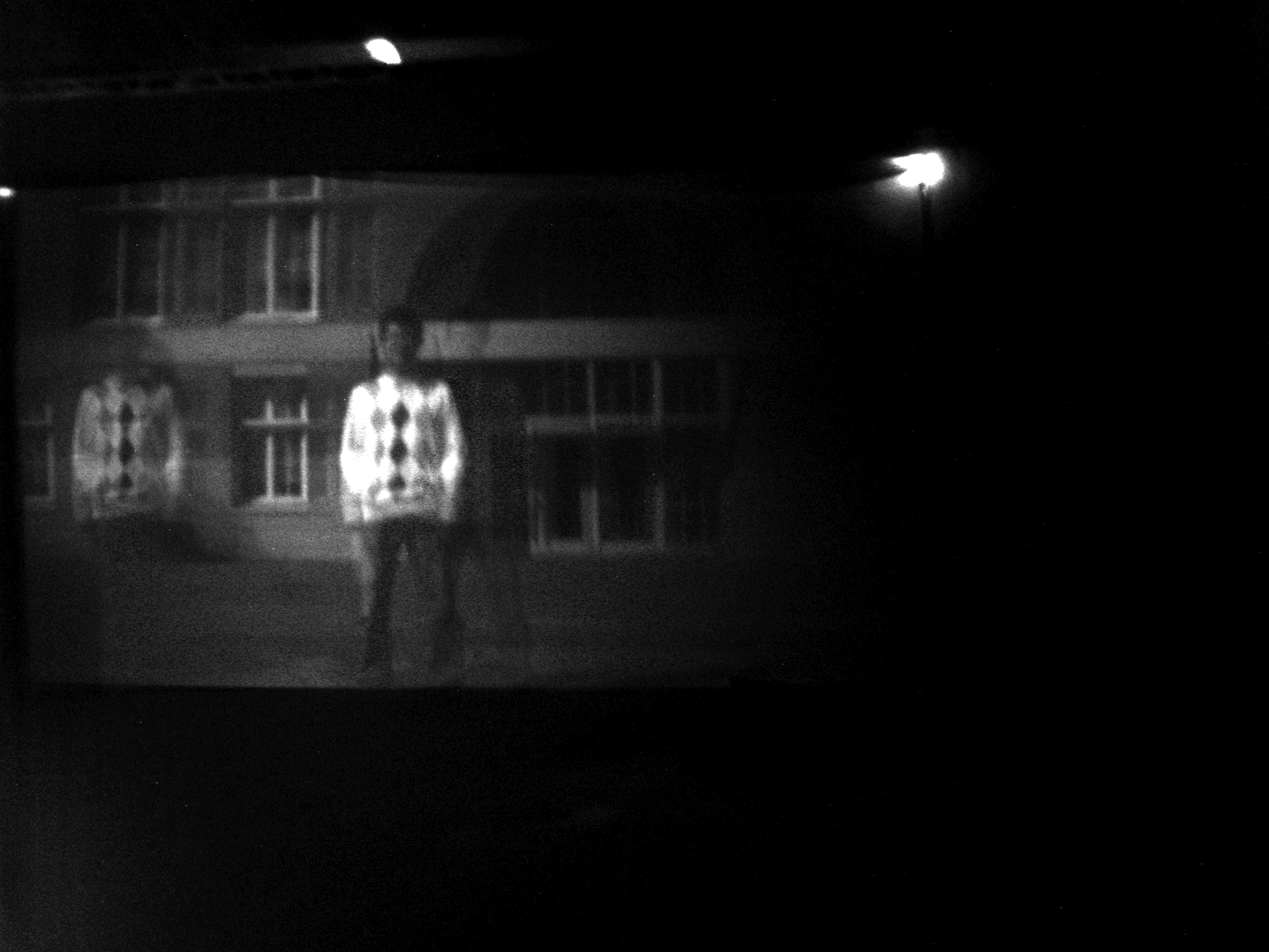
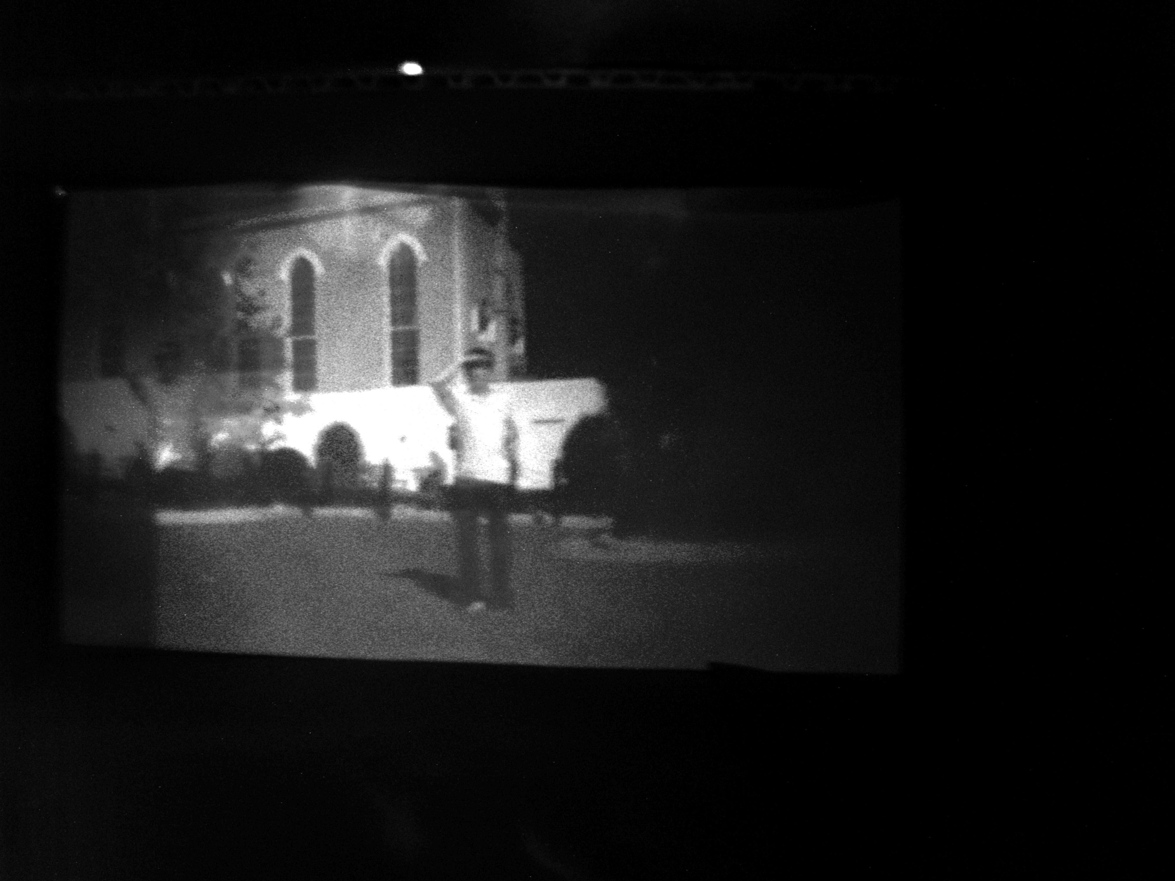
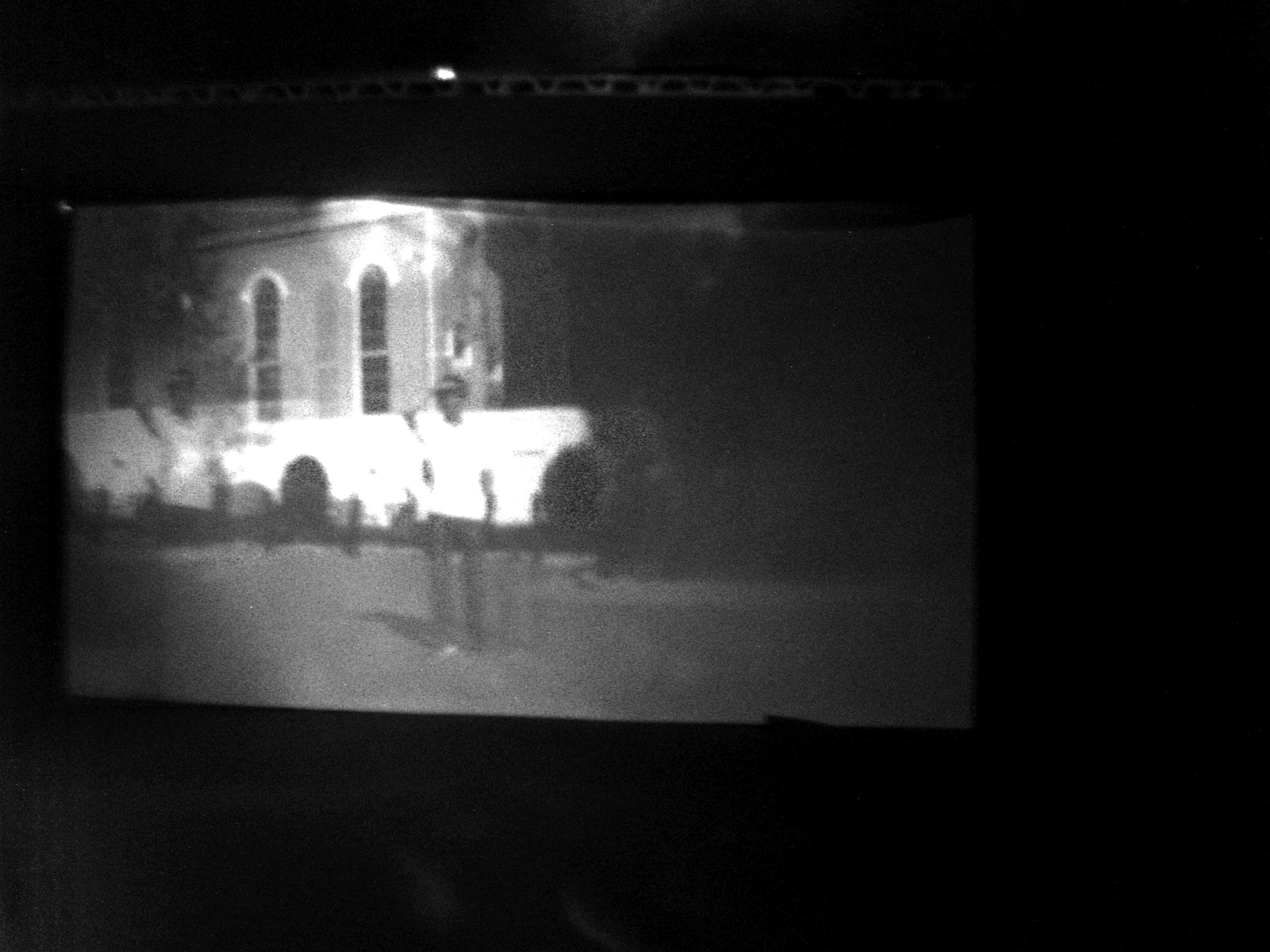
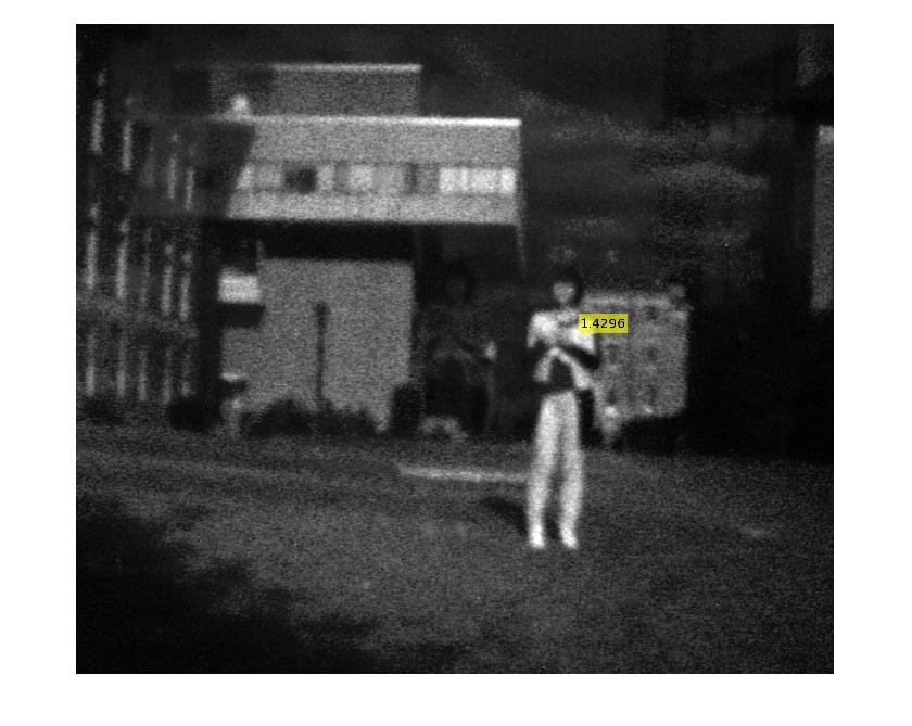
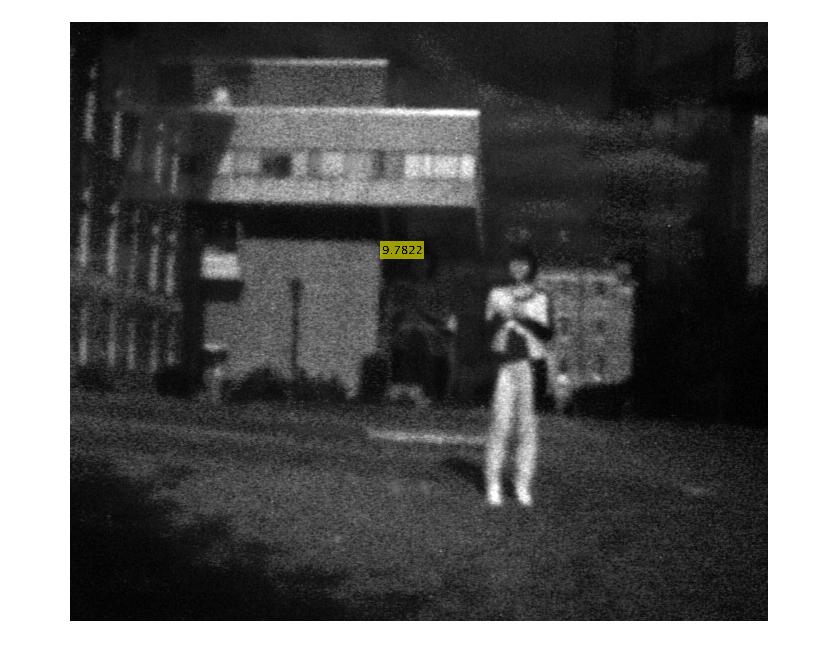
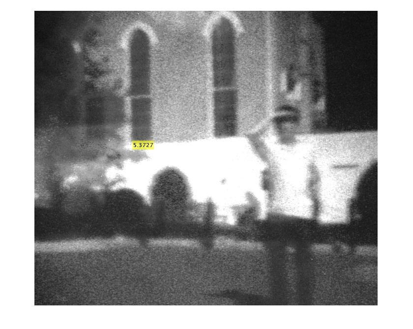
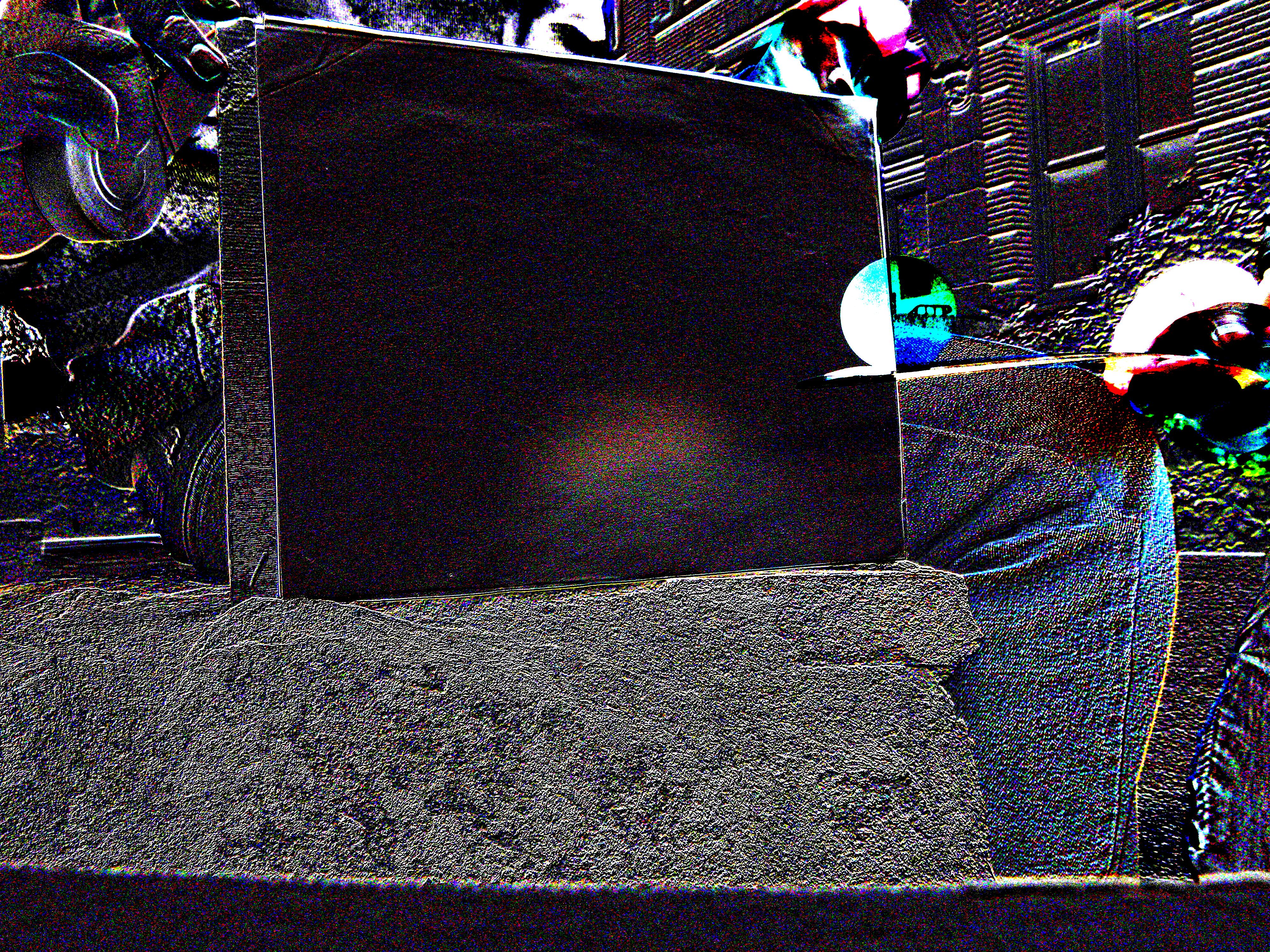
1.3 Stereo pinhole camera

The images taken were of very low quality as the maximum exposure available was 8secs hence the pinhole camera doesnt collect much light.

Fig 2 is a cropped, flipped upside down and multiplied by 10 version of the original captured image. The rest of the following images are the separate channel images.

Fig 2: Enhanced version of the pinhole image
Fig 3: Scene1 left image	Fig 3:Scene1 right image
Fig 4: Scene2 left image	Fig 4: Scene2 right image
Fig 5: Scene3 left image	Fig 5: Scene3 right image

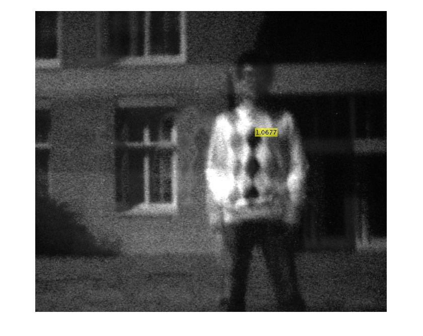
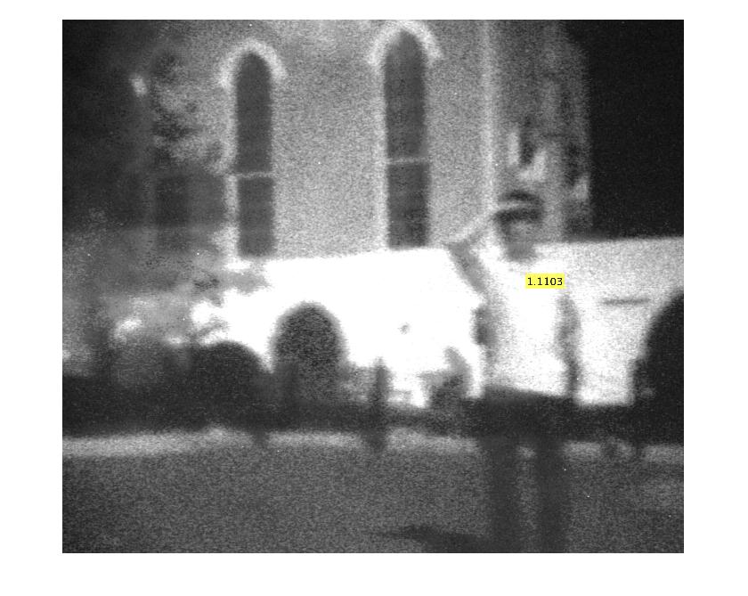
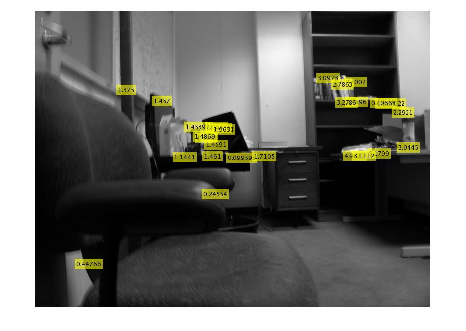
1.3.1 Manual estimation of depth using pinhole images :

The manual estimation was done using the anaglyph images. The iminfo command in MATLAB gave the focal length. In this you can specify two points interactively (ginput) and the program gives an estimation of depth at that point. Click on the image to see the estimated depths. The baseline can be estimated by taking a photo of a ruler and then doing the real-world to pixel co-ordinates conversion.

Fig 6:Depth near	Fig 6: Depth far
Fig 7: Depth near	Fig 7:Depth far
Fig 8: Depth near	Fig 8: Depth far

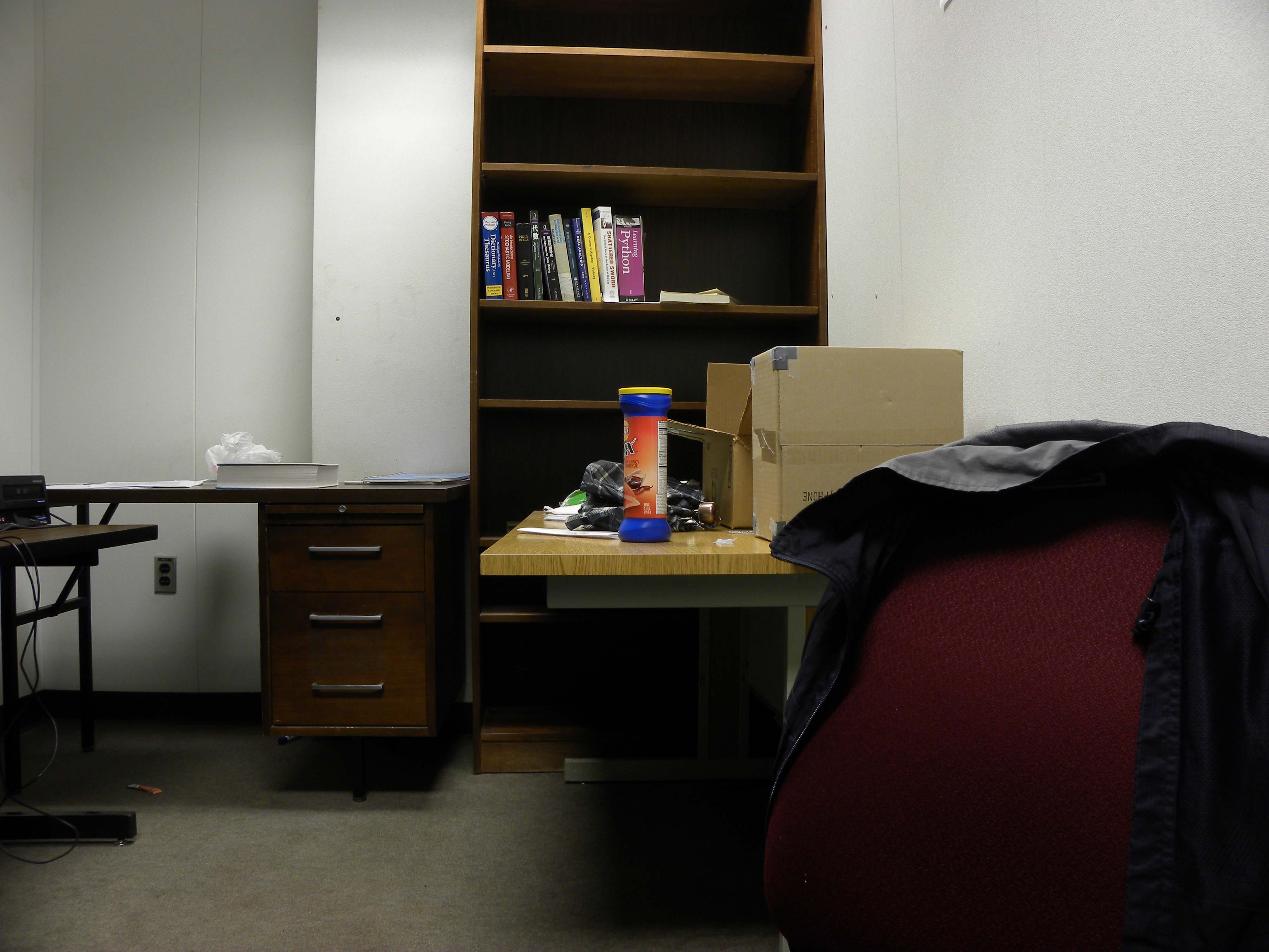
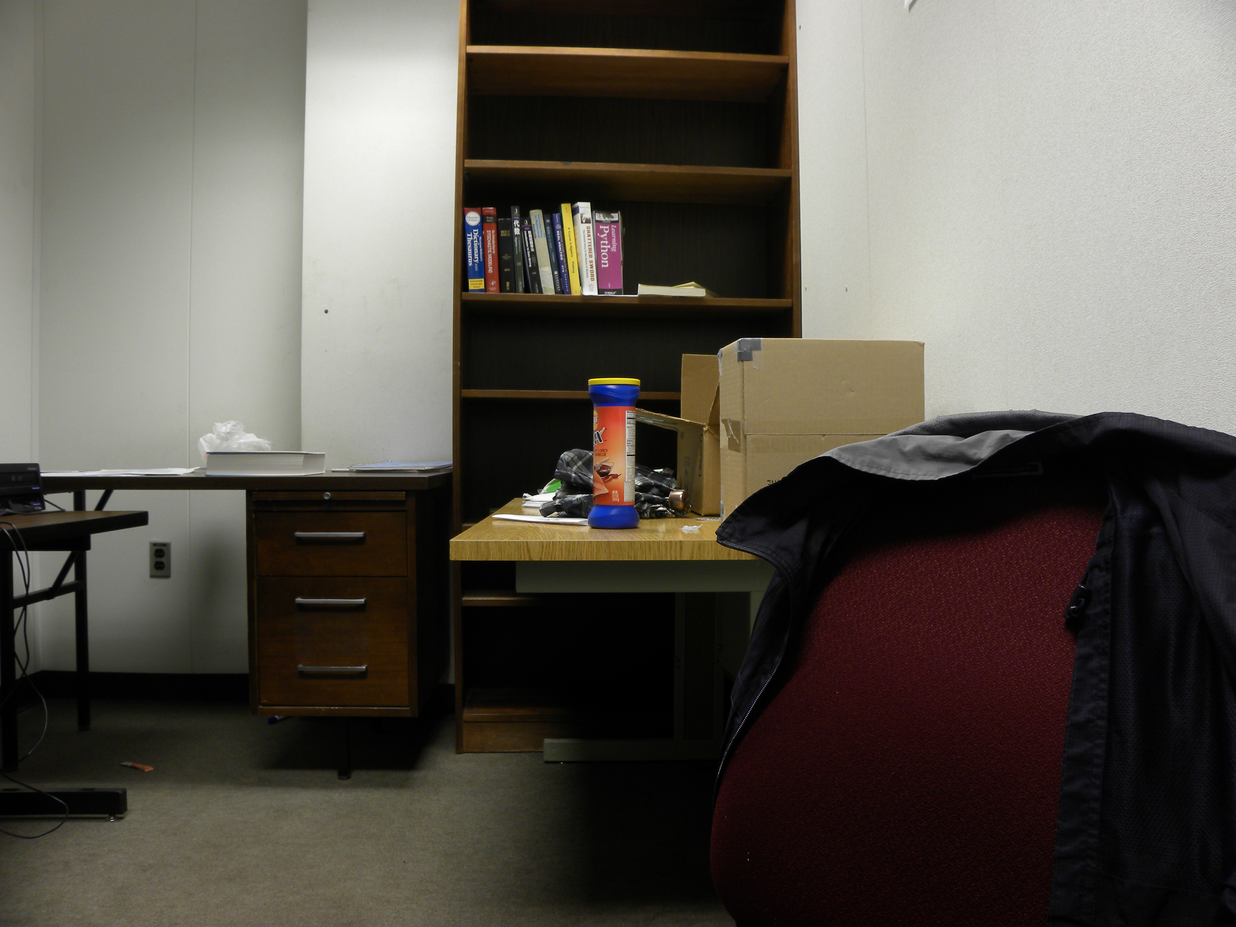
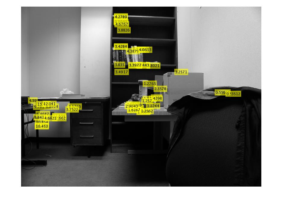
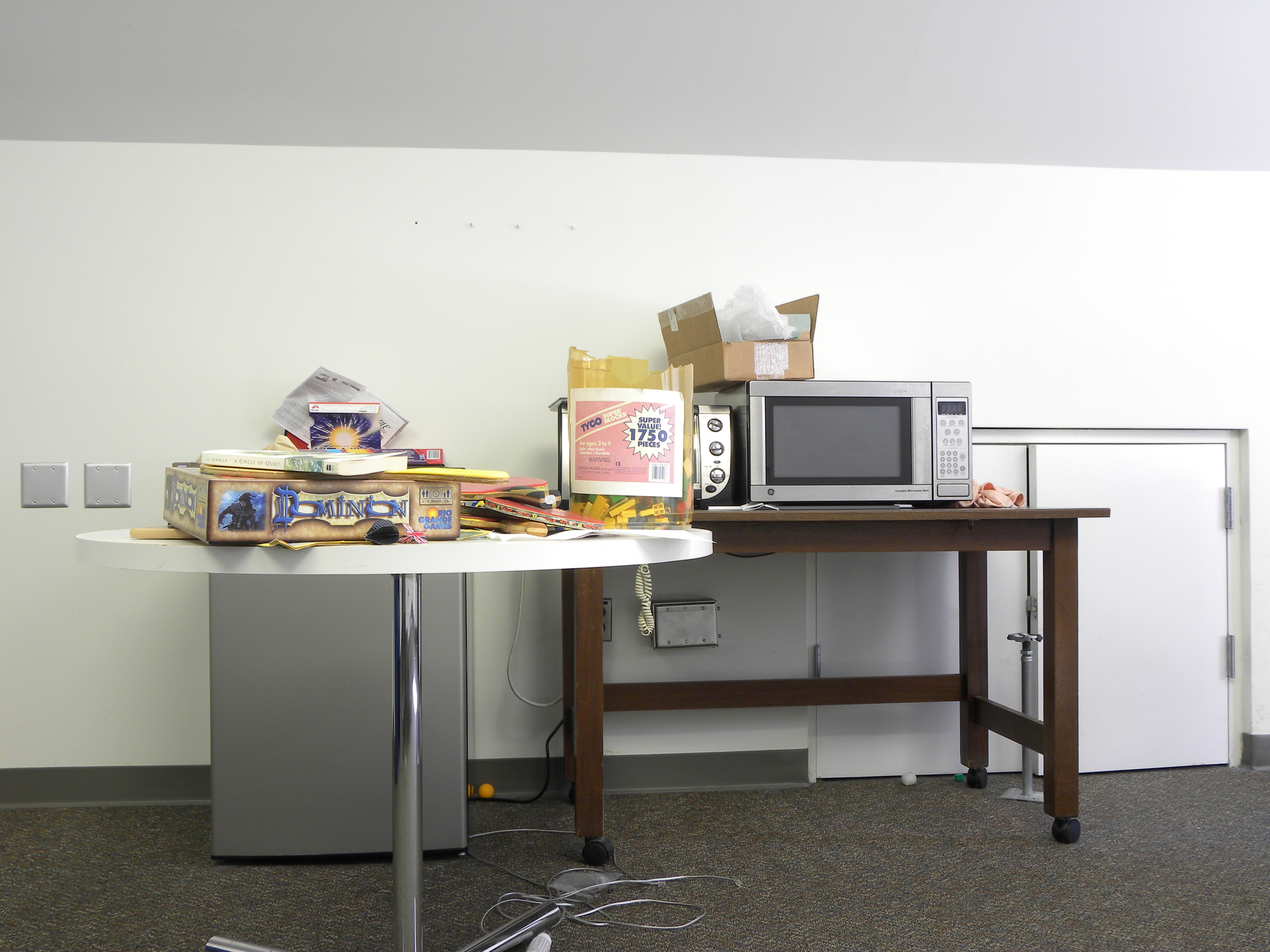
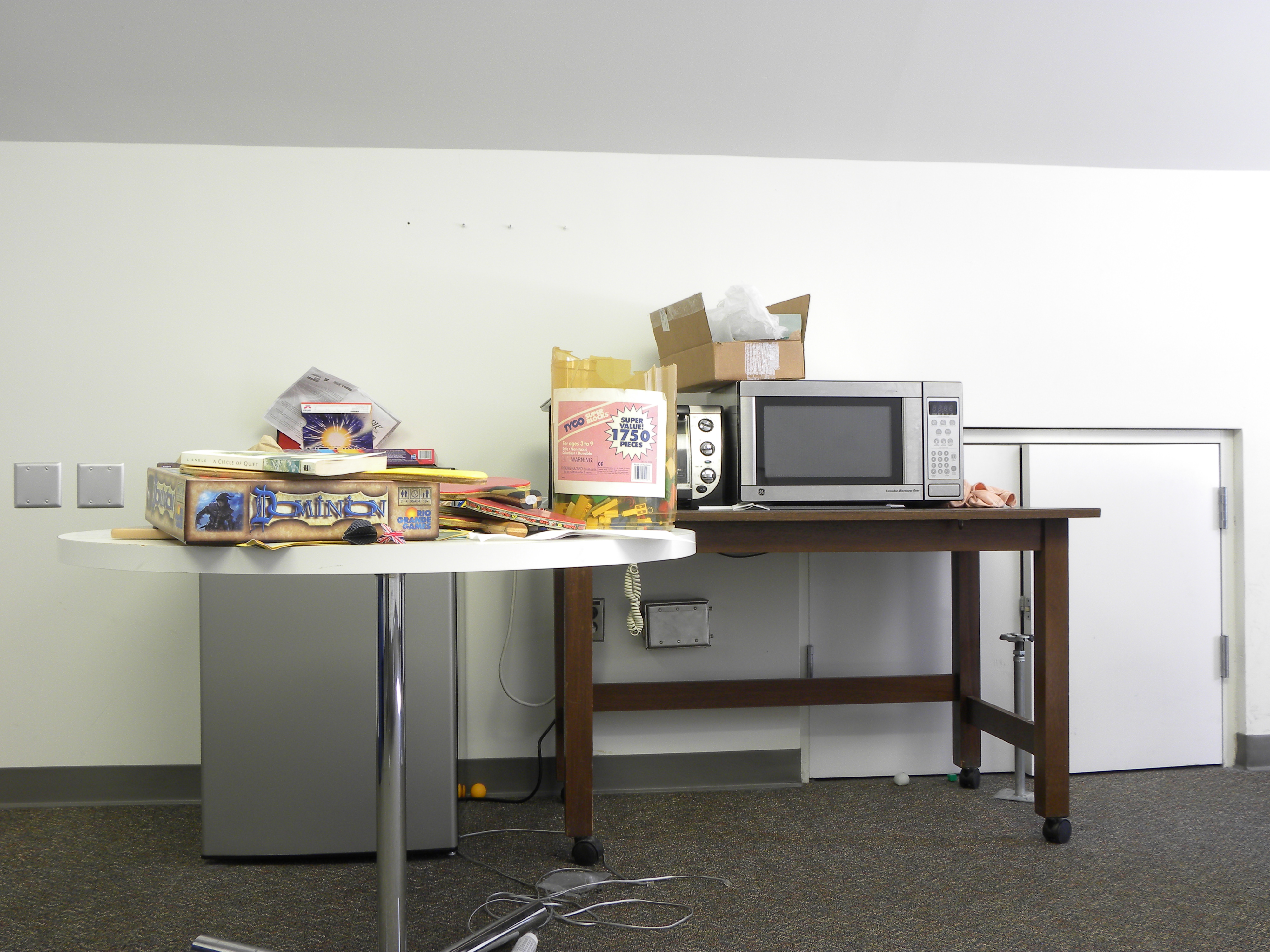
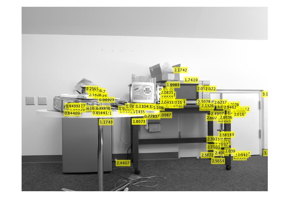
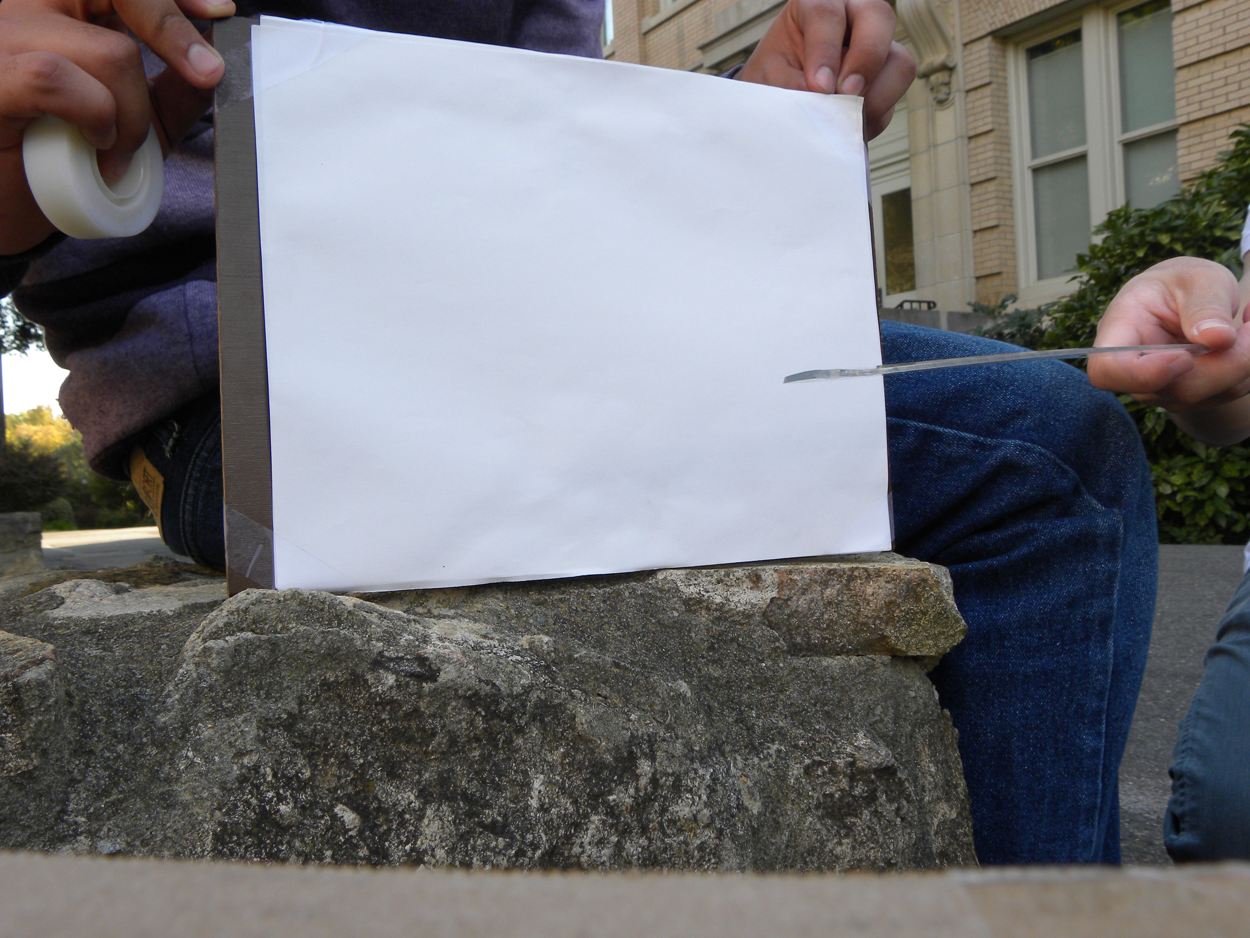
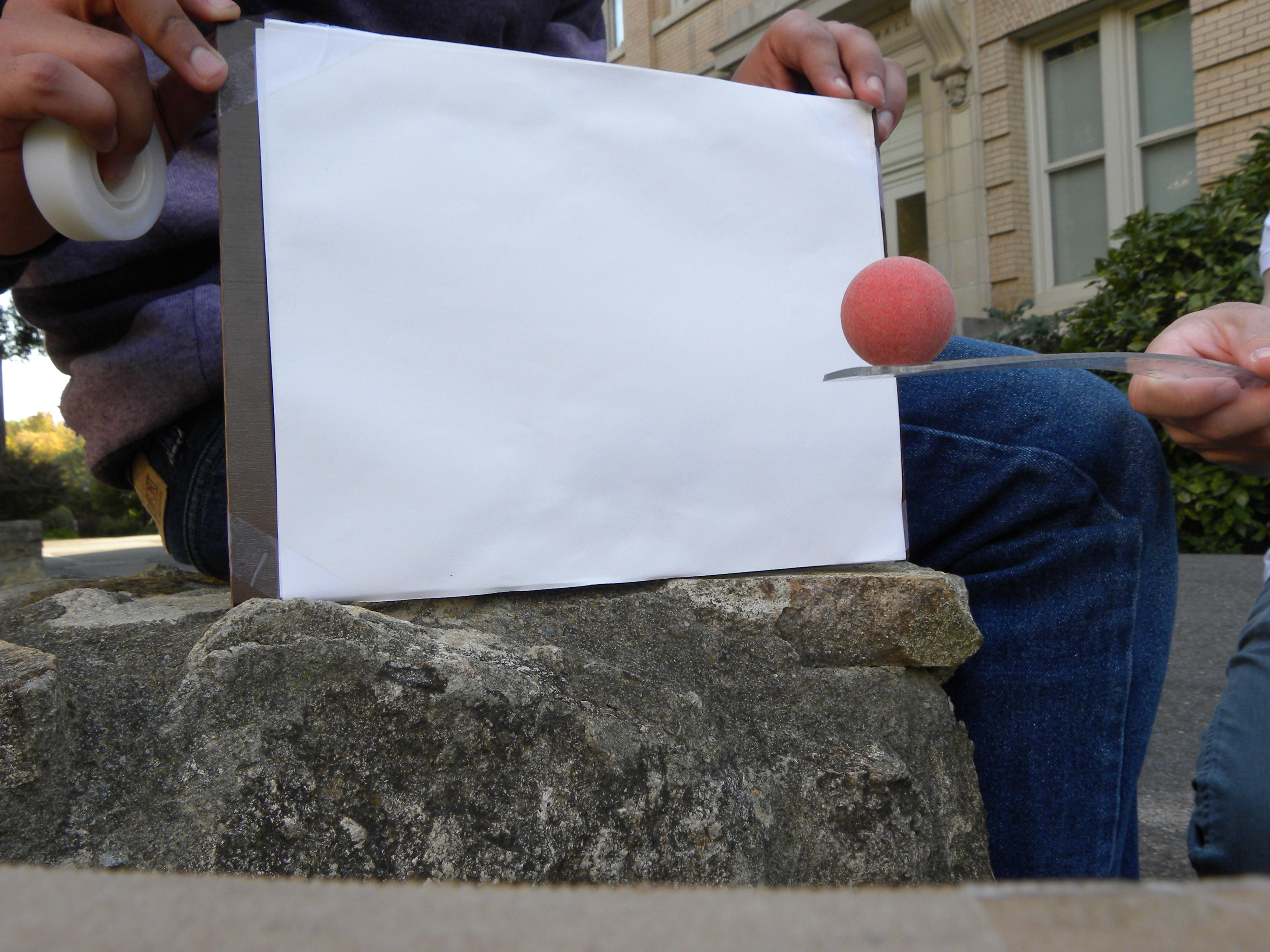
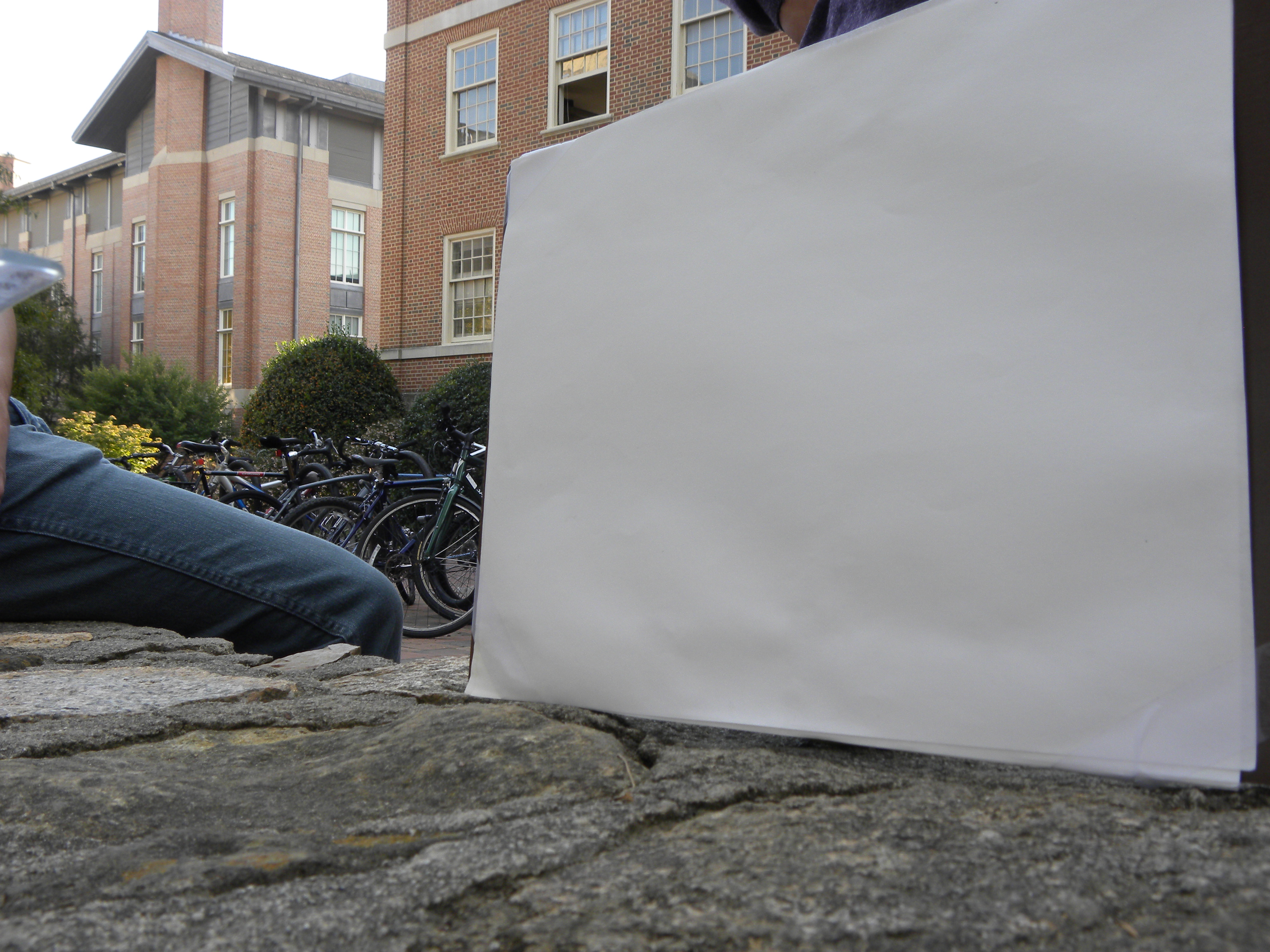
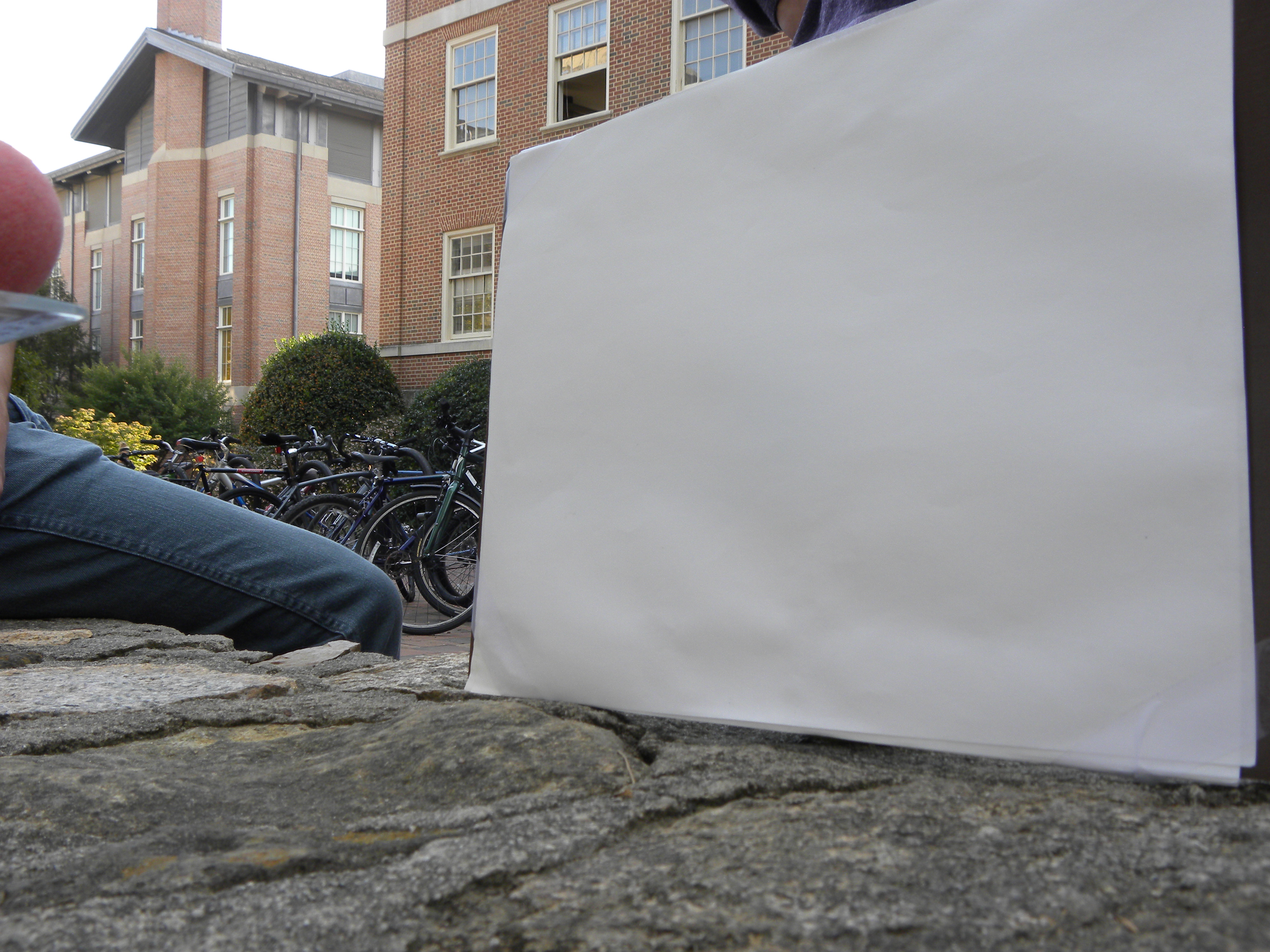
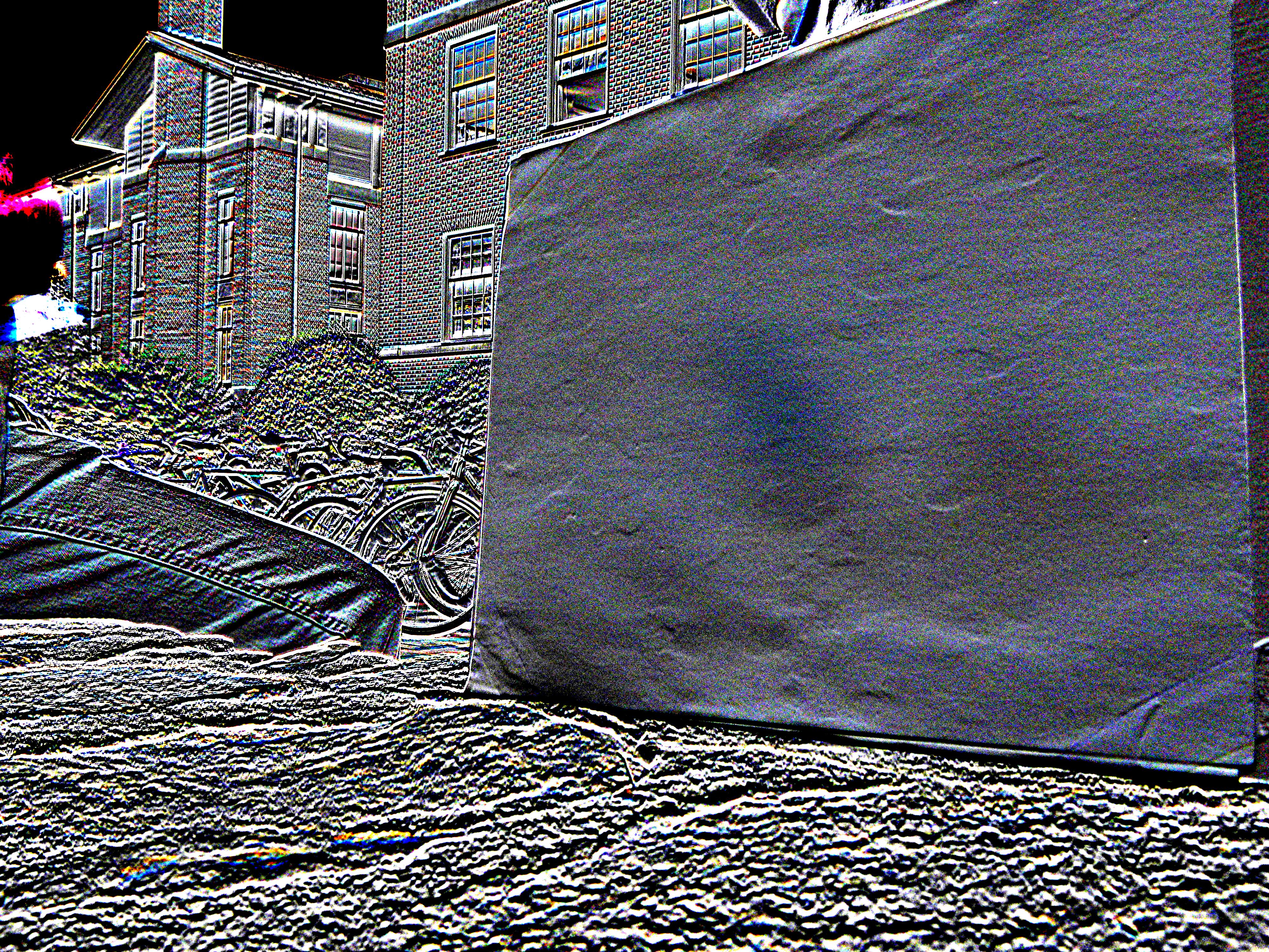
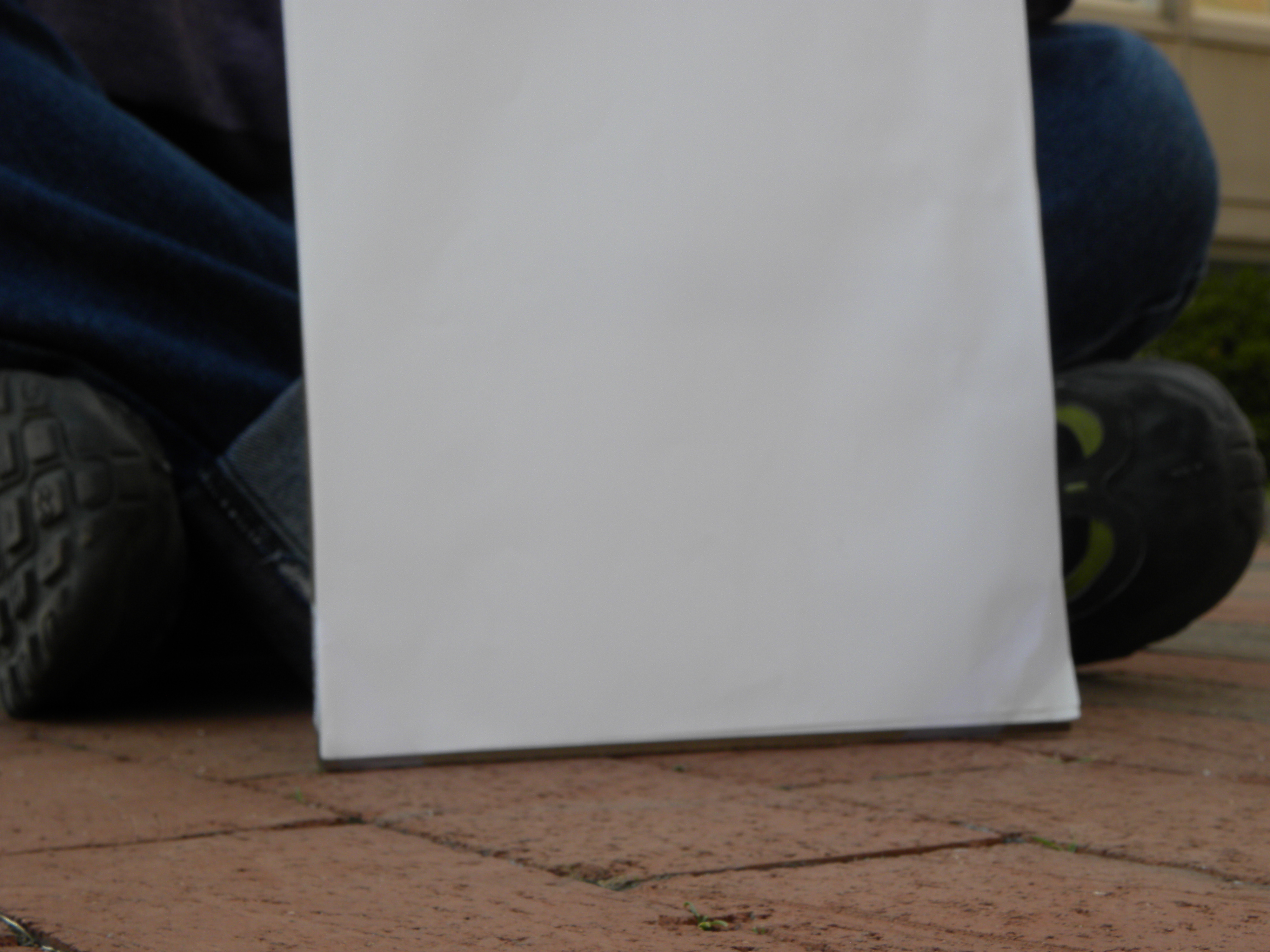
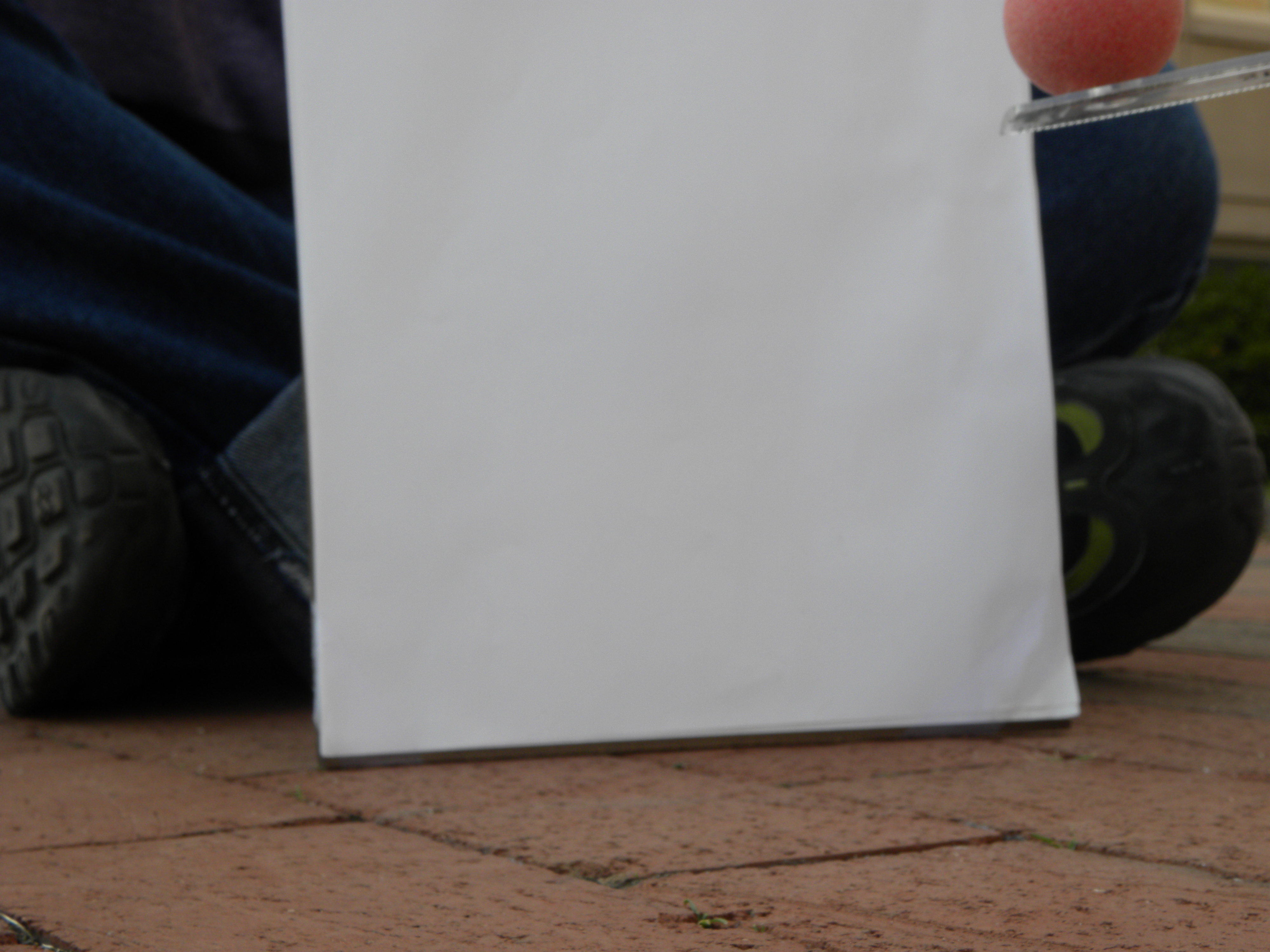
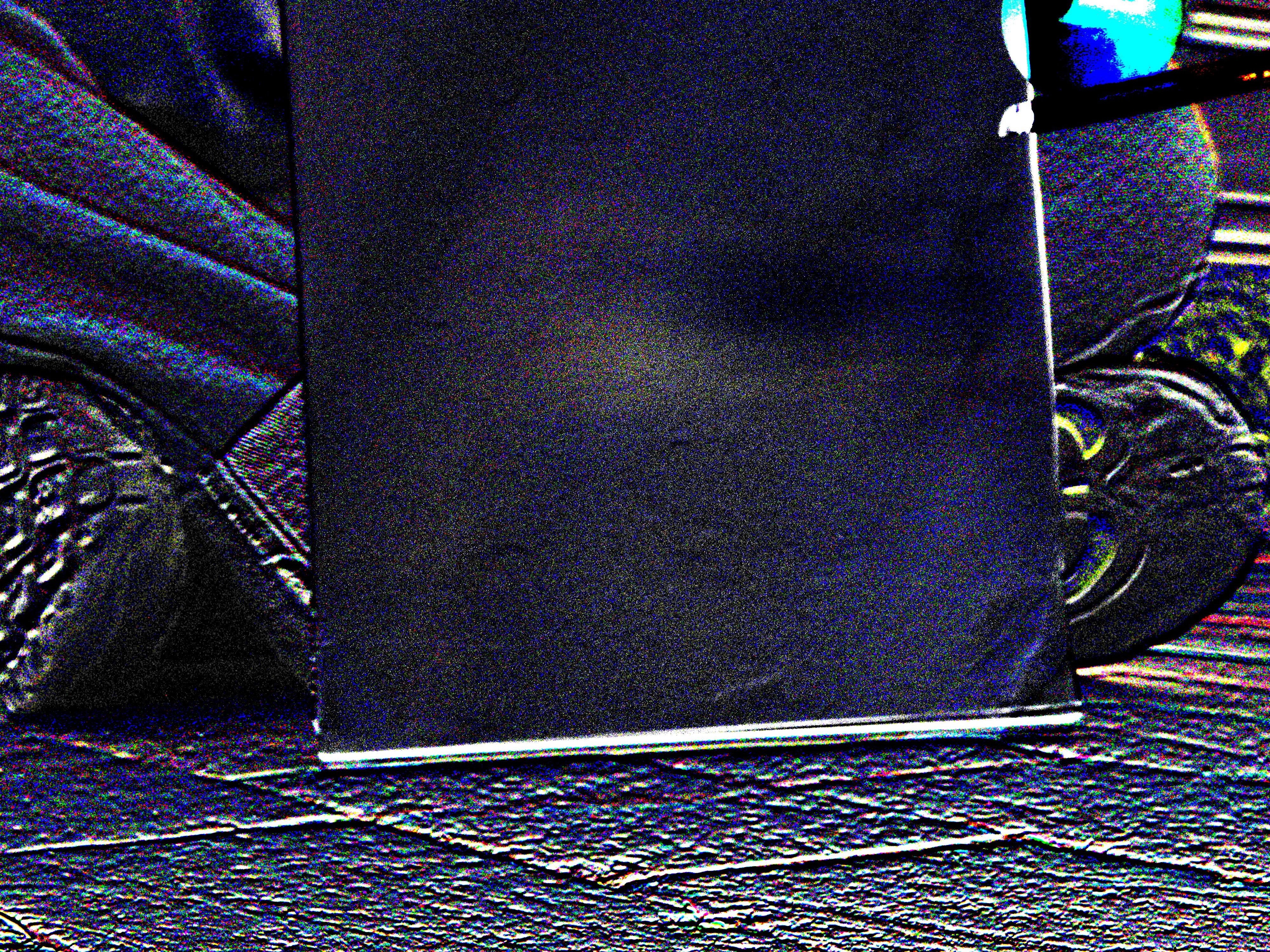
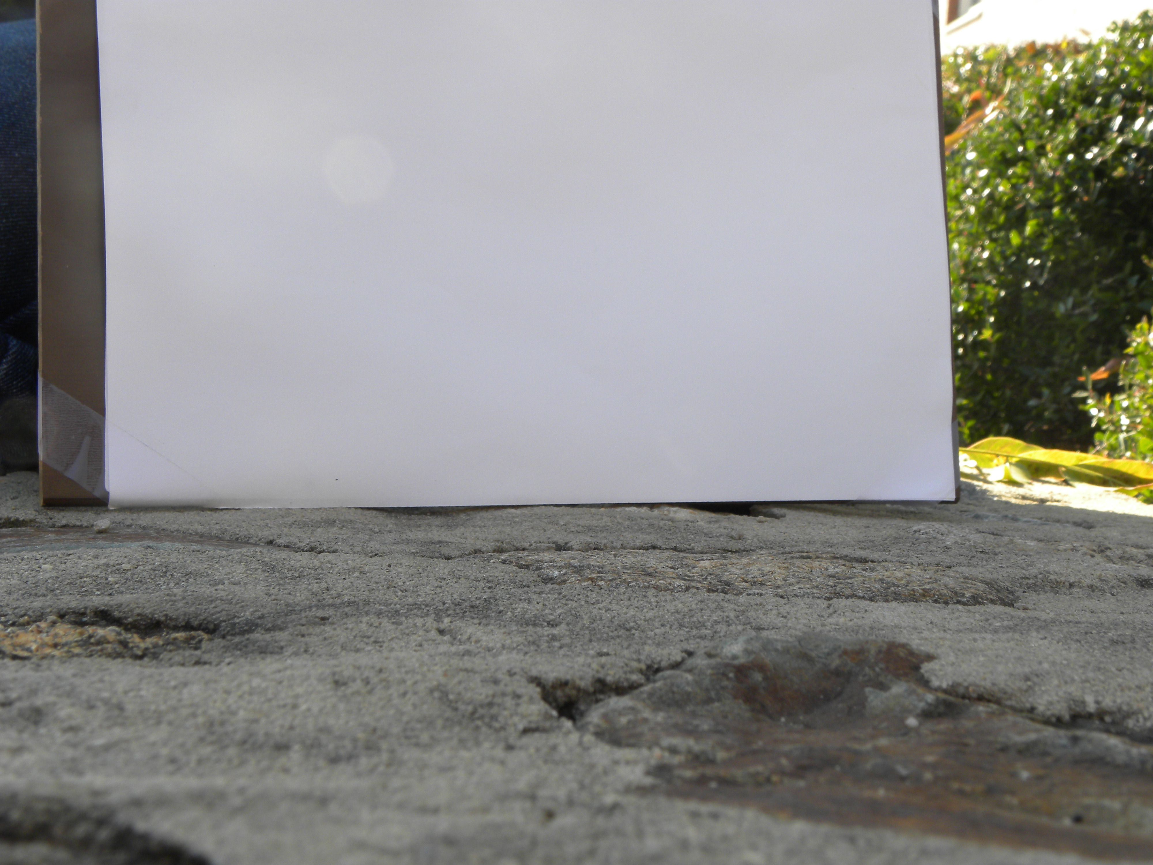
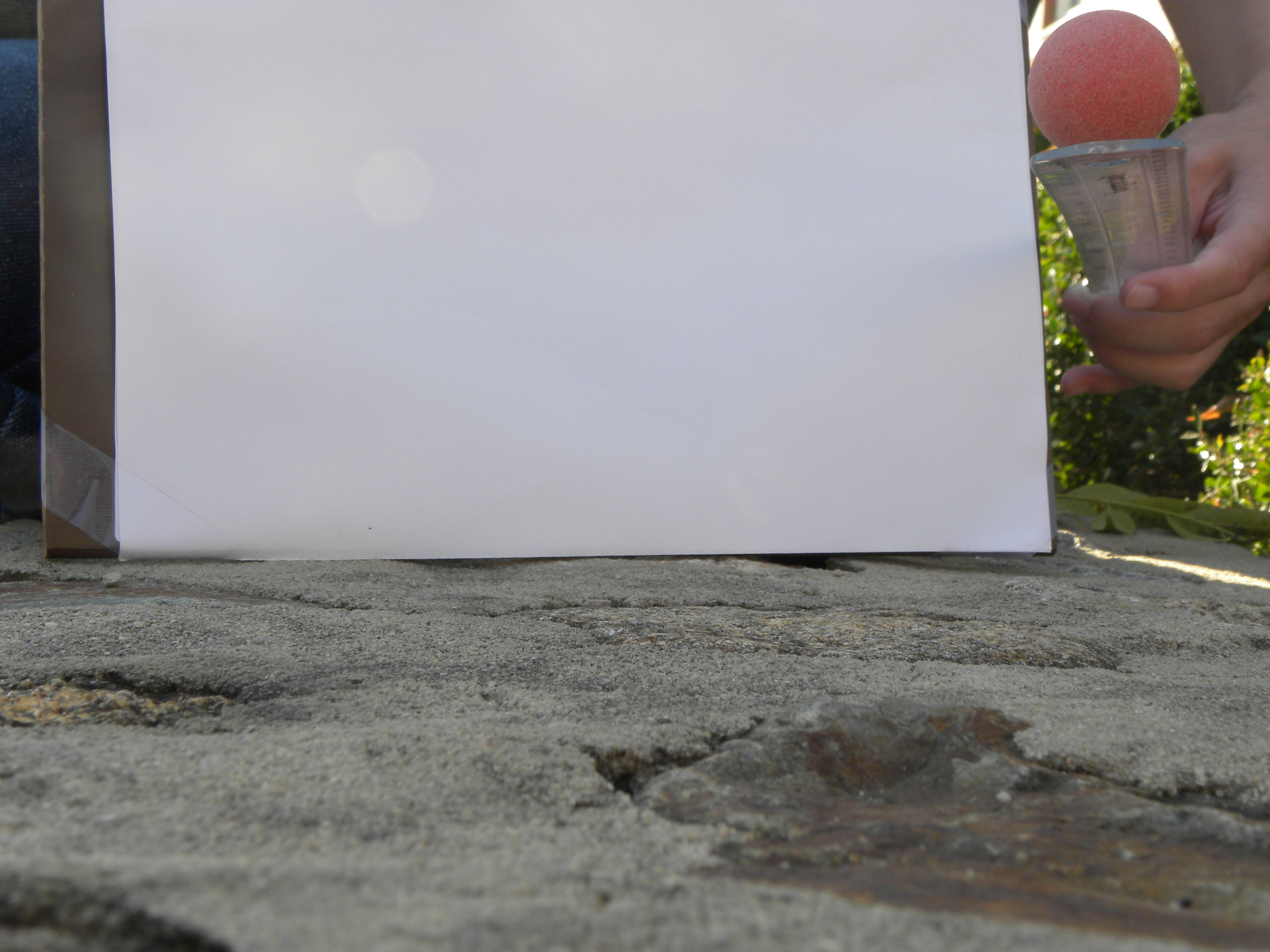
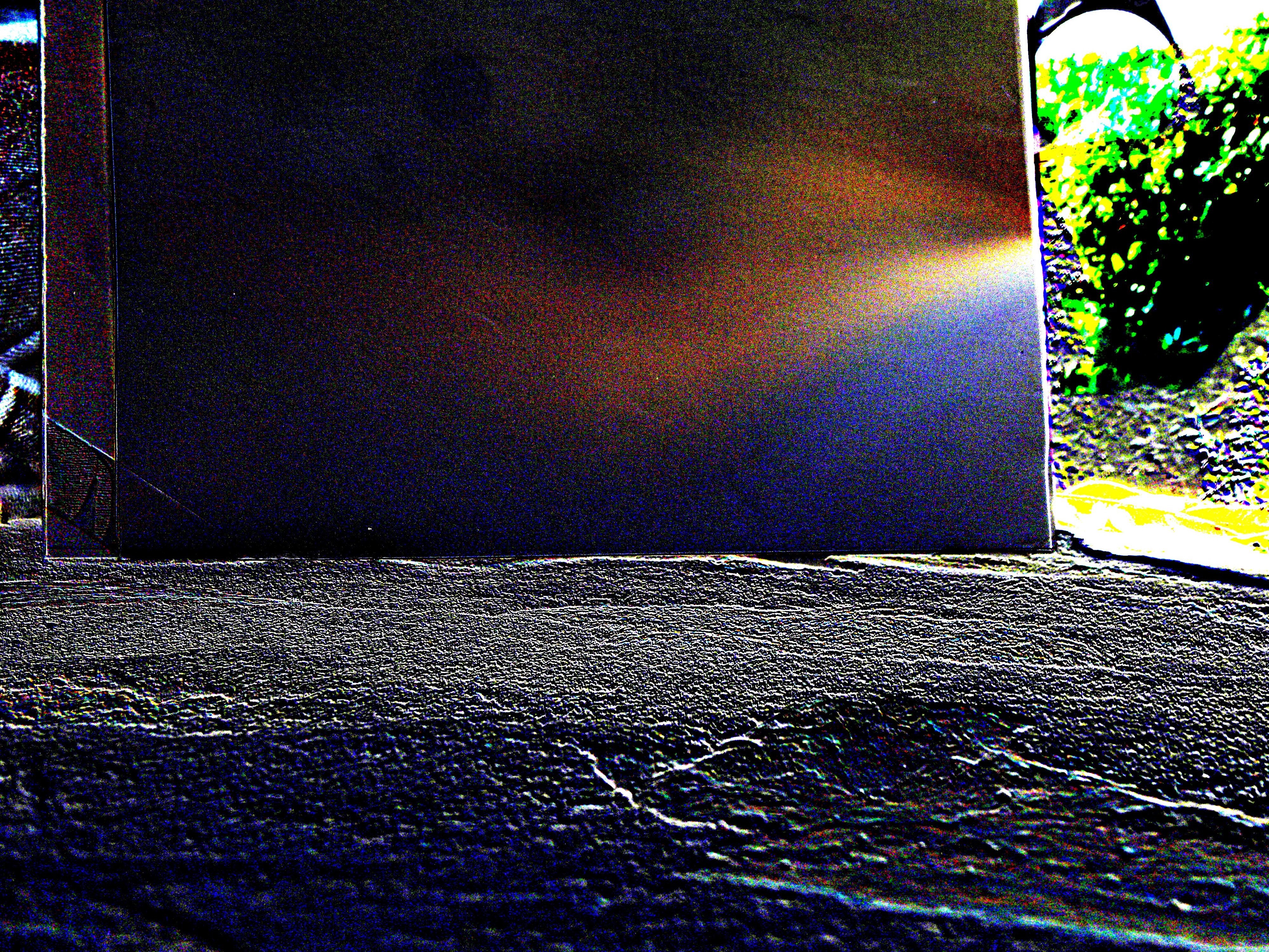
1.3.2 Automatic estimation of depth using stereo pairs

The pinhole images are very noisy to get good correspondences. Hence automatic depth estimation was done on stereo images that we captured. The Pair of images were assumed to be in the same plane and no rectification was used. This algorithm used the SURF features to get the correspondences.

Fig 9: Scene1 left image	Fig 9: Scene1 right image	Fig 9: Scene1 Estimated depths at points
Fig 10: Scene2 left image	Fig 10: Scene2 right image	Fig 10: Scene2 Estimated depths at points
Fig 11: Scene3 left image	Fig 11: Scene3 right image	Fig 11: Scene3 Estimated depths at points

1.4 Anti-pinhole images

The process of taking anti-pinhole images was the toughest. We took a white paper and taped it to a board. This functioned as our screen. With this, we used a table tennis ball as an occluder. The difference image was multiplied by a scaling factor which was adjusted on a case to case basis.

Fig 12: Background image	Fig 12: With occluder	Fig 12: Anti-pinhole image(upside down)
Fig 13: Background image	Fig 13: With occluder	Fig 13: Anti-pinhole image(upside down)	Fig 13: Actual scene
Fig 14: Background image	Fig 14: With occluder	Fig 14: Anti-pinhole image(upside down)	Fig 14: Actual scene
Fig 14: Background image	Fig 14: With occluder	Fig 14: Anti-pinhole image(upside down)	Fig 14: Actual scene