


 of
of
Since the differential equation is non-linear, the existence and
uniqueness theorem guarantees only that there is a solution in some
interval about t = 0. Suppose that we try to compute a solution of the
initial value problem on the interval  using different
numerical procedures. If we use the Euler method with
using different
numerical procedures. If we use the Euler method with  , and
, and
 , we find the following approximate values at t = 1,
 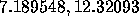 and
and  , respectively. The large differences among the computed values
are convincing evidence that we should use a more accurate
numerical procedure---the Runge-Kutta method, for example.
Using the Runge-Kutta method with
, respectively. The large differences among the computed values
are convincing evidence that we should use a more accurate
numerical procedure---the Runge-Kutta method, for example.
Using the Runge-Kutta method with  we find the approximate value
 at t = 1, which is quite different from those obtained using the
Euler method. Repeating the calculations using step sizes of
at t = 1, which is quite different from those obtained using the
Euler method. Repeating the calculations using step sizes of  and
and
 , we obtain the interesting information listed in Table 2.
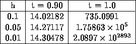
Table 2: Calculation of the Solution of the Initial Value Problem  ,
,  , using the Runge-Kutta Method
While the values at  are reasonable and we might well believe that
the solution has a value of about
are reasonable and we might well believe that
the solution has a value of about  at
at  , it is clear that
something strange is happening between
, it is clear that
something strange is happening between  and
and  . To help
determine what is happening, let's turn to some analytical approximations to
the solution of the initial value problem. Note that on
. To help
determine what is happening, let's turn to some analytical approximations to
the solution of the initial value problem. Note that on  ,
,
This suggests that the solution  of
of
and the solution  of
of
are upper and lower bounds, respectively, for the solution  of
the original problem, since all of these solutions pass through the same
initial point. Indeed, it can be shown that
of
the original problem, since all of these solutions pass through the same
initial point. Indeed, it can be shown that 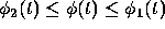 as long as these functions exist.
This is important because we can solve Eqs. (4) and (5)
analytically for  and
and  by separation of variables.
We find that
by separation of variables.
We find that

thus  as
as  , and
, and
 as
as 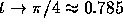 .
These calcuations show that the solution of the original initial value
problem must become unbounded somewhere between
.
These calcuations show that the solution of the original initial value
problem must become unbounded somewhere between
 and t = 1. We thus see that the problem (2) has
no solution on the entire interval
and t = 1. We thus see that the problem (2) has
no solution on the entire interval  .
.
Our numerical calculations, however, suggest that we can go beyond
 , and probably beyond
  . Assuming that the solution
of the initial value problem exists at
. Assuming that the solution
of the initial value problem exists at  and has the value
  ,
we can obtain a more accurate appraisal of what happens for larger t
by considering the initial value problems (4) and (5)
with
,
we can obtain a more accurate appraisal of what happens for larger t
by considering the initial value problems (4) and (5)
with  replaced by
  . Then we obtain

where only four decimal places have been kept. Thus
 as
as 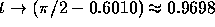 and
and  as
as  .
We conclude that the solution of the initial value problem (2)
becomes unbounded near
.
We conclude that the solution of the initial value problem (2)
becomes unbounded near  . We cannot be more precise because
the initial condition
. We cannot be more precise because
the initial condition  is only approximate. This example
illustrates the sort of information that can be obtained by a
judicious combination of analytical and numerical work.
is only approximate. This example
illustrates the sort of information that can be obtained by a
judicious combination of analytical and numerical work.


